Spontaneous and Dynamical Scalarization

Scalarization produces a nonlinear scalar profile rather than merely a large weak-field response. In a continuous transition, a compact object’s GR branch develops a regular static zero mode; beyond that onset, nonlinear terms can saturate the instability on a branch with a finite scalar profile and charge. Discontinuous transitions can instead admit finite-amplitude scalarized states while the GR branch remains locally stable. The linear onset is an eigenvalue problem, the scalarized object is a nonlinear boundary-value problem, and dynamical or induced scalarization is an evolution problem. Keeping those three calculations separate is essential for reproducibility and for judging stability.

Required background. Einstein Equations supplies the GR compact-star branch about which the scalar is perturbed.

Helpful background. Gravitational Actions and Boundary Terms supplies the variational and asymptotic data for the scalar; Formulations of General Relativity supplies the constraint and boundary-value formulation; Gravity Beyond General Relativity supplies the branch, cutoff, and independent-check criteria; Relativistic Matter and Compact Objects supplies the stellar equation of state, regular center, surface matching, and baryon-mass controls used in a full calculation.

A tachyonic mode on the GR branch

Use the Einstein-frame action

$$S=\frac{1}{16\pi G_*}\int d^4x\sqrt{-g_*} \left[R_*-2(\nabla_*\varphi)^2\right] +S_m[A^2(\varphi)g^*_{ab},\psi].$$

The scalar equation is

$$\Box_*\varphi=-4\pi G_*\alpha(\varphi)T_*, \qquad \alpha(\varphi)=\frac{d\ln A}{d\varphi}.$$

For the symmetric coupling

$$A(\varphi)=\exp\left(\frac12\beta\varphi^2\right), \qquad \alpha(\varphi)=\beta\varphi,$$

$\varphi=0$ is a GR branch. Linearizing on a GR stellar background gives

$$(\Box_*-m_{\mathrm{eff}}^2)\delta\varphi=0, \qquad m_{\mathrm{eff}}^2=-4\pi G_*\beta T_*.$$

For ordinary stellar matter $T_*\simeq-\rho_*+3p_*$. A sufficiently negative $\beta$ can make $m_{\mathrm{eff}}^2\lt0$ over a large enough region. That is a tachyonic, infrared instability: the lowest spatial eigenvalue crosses zero before a static perturbation grows into a nonlinear profile. The general tachyonic mechanism and its compact-star realization are reviewed in Doneva et al. 2024, §§ II.A–II.B, equations (1)–(16).

The sign of a local effective mass is not by itself the onset criterion. A finite star supplies a gradient energy and exterior matching condition. One must solve the global zero-mode problem with regular center data and decay at infinity.

A solvable zero-mode benchmark

Take a Newtonian constant-density star of radius $R$, neglect pressure in $T\simeq-\rho$, and let the scalar be massless outside. For a static spherical mode define $u=r\,\delta\varphi$ and $x=r/R$. Inside,

$$\frac{d^2u}{dx^2}+\kappa^2u=0, \qquad \kappa^2=-4\pi G_*\beta\rho R^2\gt0.$$

Regularity gives $u(0)=0$. Outside, asymptotic decay $\delta\varphi=Q/r$ makes $u$ constant, so surface matching gives $u'(1)=0$. The regular interior solution $u=\sin(\kappa x)/\kappa$ then obeys

$$\cos\kappa=0, \qquad \kappa_c=\frac{\pi}{2}$$

for the first mode. Equivalently, with compactness $\mathcal C=G_*M/R=4\pi G_*\rho R^2/3$,

$$\beta_c=-\frac{\pi^2}{12\mathcal C}.$$

This is a teaching benchmark, not a realistic neutron-star threshold. It isolates the eigenvalue, boundary condition, and sign checks that a relativistic solver must reproduce.

Recomputed convergence

The retained reference calculation used CPython 3.9.6, NumPy 2.0.2, and SciPy 1.13.1 in double precision. A fixed-step fourth-order Runge–Kutta shooting method integrates $u''=-\kappa^2u$; Brent bracketing finds $u'(1)=0$. The analytic Rayleigh quotient

$$\kappa_{\mathrm{var}}^2 =\frac{\int_0^1(u')^2dx}{\int_0^1u^2dx} =\frac{\pi^2}{4}, \qquad u=\sin\left(\frac{\pi x}{2}\right),$$

is the independent benchmark. The finite-difference residual in the last column evaluates the differential equation independently on the stored RK4 samples.

Steps $N$	Eigenvalue $\kappa_N$	Error $\lvert\kappa_N-\pi/2\rvert$	Boundary mismatch $\lvert u'(1)\rvert$	Independent FD residual
16	1.570797538629	1.212e-6	9.71e-17	1.258e-3
32	1.570796402730	7.594e-8	3.47e-17	3.152e-4
64	1.570796331544	4.749e-9	1.46e-16	7.884e-5
128	1.570796327092	2.969e-10	4.68e-17	1.971e-5

The eigenvalue error falls by about $2^4$ per doubling, as expected for RK4. The independently sampled second-difference residual falls by about $2^2$. A tiny shooting mismatch alone would not demonstrate convergence; it only shows that the discrete shooting equation was solved accurately.

The executable source is below. Saving the program as scalarization_zero_mode.py preserves the exact reference calculation. The program must produce the four refinement rows, verify the pinned environment, and exit nonzero if either convergence trend fails.

import argparse
import math
import sys
from importlib.metadata import version

import numpy as np
from scipy.optimize import brentq


def shoot(kappa, steps):
    h = 1.0 / steps
    y = np.array([0.0, 1.0])  # u(0), u'(0)
    samples = [float(y[0])]

    def rhs(state):
        return np.array([state[1], -(kappa * kappa) * state[0]])

    for _ in range(steps):
        k1 = rhs(y)
        k2 = rhs(y + 0.5 * h * k1)
        k3 = rhs(y + 0.5 * h * k2)
        k4 = rhs(y + h * k3)
        y += h * (k1 + 2 * k2 + 2 * k3 + k4) / 6.0
        samples.append(float(y[0]))
    return float(y[1]), np.asarray(samples)


def solve(steps):
    root = brentq(lambda k: shoot(k, steps)[0], 1.0, 2.0,
                  xtol=5e-15, rtol=1e-14)
    boundary, u = shoot(root, steps)
    h = 1.0 / steps
    residual = np.max(np.abs(
        (u[2:] - 2 * u[1:-1] + u[:-2]) / h**2
        + root**2 * u[1:-1]
    ))
    return root, abs(root - math.pi / 2), abs(boundary), float(residual)


def main():
    parser = argparse.ArgumentParser()
    parser.add_argument('--check', action='store_true')
    parser.parse_args()
    assert sys.version_info[:3] == (3, 9, 6)
    assert version('numpy') == '2.0.2'
    assert version('scipy') == '1.13.1'
    rows = [(n, *solve(n)) for n in (16, 32, 64, 128)]
    for row in rows:
        print(row[0], *(f'{value:.12e}' for value in row[1:]))
    errors = [row[2] for row in rows]
    residuals = [row[4] for row in rows]
    assert all(b < a for a, b in zip(errors, errors[1:]))
    assert all(b < a for a, b in zip(residuals, residuals[1:]))


if __name__ == '__main__':
    main()

Run it from the directory in which it was saved:

python3 -c "import sys,numpy,scipy; print(sys.version.split()[0],numpy.__version__,scipy.__version__)"
python3 scalarization_zero_mode.py
python3 scalarization_zero_mode.py --check

Continuing the nonlinear branch

The zero mode locates a bifurcation but does not supply the scalarized star. A full relativistic calculation integrates the coupled stellar equations for mass, lapse, pressure, scalar, and scalar derivative. Regular center series set $m(0)=0$ and $\varphi'(0)=0$; the stellar surface is found from $p(R)=0$; the exterior is integrated until

$$\varphi(r)=\varphi_\infty+\frac{Q}{r}+O(r^{-2}).$$

In this normalization the tail coefficient is $Q=-G_*m_A\alpha_A$, where $\alpha_A=\partial\ln m_A/\partial\varphi_\infty$ at fixed baryon number. Thus $Q$ is a length, whereas $\alpha_A$ is a dimensionless coupling; their signs are opposite for positive mass. This conversion is needed when the stellar solution is used in the radiation formulas.

One shoots on the central scalar value to reach the prescribed $\varphi_\infty$ while holding central density, baryon mass, or another named control fixed. Pseudo-arclength continuation is needed near a fold, where stepping only in $\beta$ or central density can jump branches. Damour and Esposito-Farèse give the stellar system and matching variables in Damour and Esposito-Farèse 1996, § III, equations (3.6a)–(3.6h).

Near onset, a reduced energy can be organized as

$$\Delta E(A_s) =\frac12\lambda_0(\beta)A_s^2 +\frac14g_4A_s^4+\frac16g_6A_s^6+\cdots.$$

When the lowest eigenvalue $\lambda_0$ crosses zero, $g_4\gt0$ gives a continuous branch with $A_s^2\simeq-\lambda_0/g_4$. If $g_4\lt0$ and $g_6\gt0$, multiple local extrema and hysteresis can appear. The coefficients must come from the full stellar theory; this normal form explains why linear onset alone cannot decide nonlinear saturation or branch stability.

For a concrete comparison, rescale the energy and amplitude to dimensionless variables. With $g_4=1$, $g_6=0$, the extrema are $A_s=0$ and $A_s=\pm\sqrt{-\lambda_0}$ for $\lambda_0\lt0$. The second derivative of the energy is $\lambda_0$ on the GR branch and $-2\lambda_0$ on the nonzero branches, explaining the exchange of stability at the continuous onset. With $g_4=-1$, $g_6=1$, put $y=A_s^2$. Nonzero extrema instead satisfy

$$y_\pm=\frac{1\pm\sqrt{1-4\lambda_0}}{2}, \qquad \Delta E''=2y(2y-1).$$

For $0\lt\lambda_0\lt1/4$, the GR state and the two outer scalarized states are local minima, separated by the inner unstable branches. The outer and inner branches meet at folds at $\lambda_0=1/4$, while the GR state loses local stability only at $\lambda_0=0$. Their energies are equal at $\lambda_0=3/16$, where $y=3/4$. A slowly driven, dissipative system can therefore remain in a metastable minimum and jump at different control values on the return path. The normal form alone does not specify those dynamics or the lifetime of a metastable star. Its stability test concerns the amplitude $A_s$ only; other stellar modes must be checked separately. The continuous Landau analogy and the distinction between charge and response are developed in Damour and Esposito-Farèse 1996, § II, equations (2.1)–(2.4), PDF.

The figure compares these two normal forms. Follow a vertical slice through the shaded interval in the lower panel: the zero-amplitude minimum and two nonzero minima coexist at the same control parameter, with unstable extrema between them. The figure uses $A$ for the rescaled amplitude $A_s$.

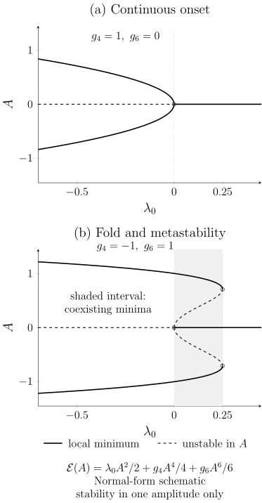
Equilibria of the dimensionless one-amplitude energy $\mathcal E(A)=\lambda_0A^2/2+g_4A^4/4+g_6A^6/6$. Solid branches are local minima and dashed branches are unstable in $A$; open circles have zero quadratic curvature and require the higher-order terms. Panel (a) has $g_4=1$, $g_6=0$. Panel (b) has $g_4=-1$, $g_6=1$, with coexisting minima for $0\lt\lambda_0\lt1/4$ and equal minimum energies at $\lambda_0=3/16$. These are analytic normal-form schematics, with no stellar data or claim about stability in other modes.

At least three mesh or tolerance refinements should be reported for the nonlinear fields, scalar charge, mass, surface location, and field-equation residuals. The onset must agree with an independent linear eigenvalue or Rayleigh calculation. A first-law or fixed-baryon-mass comparison supplies a further branch check.

Spontaneous, induced, and dynamical scalarization

Spontaneous scalarization names nonzero scalar equilibria available to an isolated object without an externally imposed scalar source; a continuous onset is the instability just analyzed, while a discontinuous transition needs the additional nonlinear branch analysis. Induced scalarization occurs when the companion’s field moves an otherwise weakly scalarized body onto a charged branch. Dynamical scalarization is the time-dependent transition during an evolving binary or collapse. A static sequence can suggest where a transition is possible, but it cannot determine its rate, radiation, or hysteresis without solving the evolution equations.

Failure modes include selecting the wrong stellar branch, underresolving the surface or a thin scalar layer, mistaking a Newton update norm for an equation residual, losing asymptotic accuracy in $Q$, and crossing a region where the scalar–tensor equations cease to be hyperbolic or the EFT cutoff is violated. Published branch existence is not a substitute for those checks.

Exercises

Derive the constant-density threshold above. Match the regular interior mode to a decaying exterior, obtain $\kappa_c=\pi/2$, and express the critical $\beta$ in terms of compactness $\mathcal C=G_*M/R$.

Solution

Inside the star, regularity selects

$$u_{\mathrm{in}}(x)=B\sin(\kappa x).$$

Outside, $\nabla^2\delta\varphi=0$ and decay gives $\delta\varphi=Q/r$, so $u_{\mathrm{out}}=Q$ is constant. Continuity of the field and its normal derivative is equivalent to continuity of $u$ and $u'$; therefore

$$u'_{\mathrm{in}}(1)=B\kappa\cos\kappa=0.$$

The trivial $B=0$ solution is excluded when looking for a zero mode, and $\kappa\gt0$, so $\cos\kappa=0$. The lowest node-free mode has $\kappa_c=\pi/2$. Since

$$\kappa_c^2=-4\pi G_*\beta_c\rho R^2$$

and a constant-density star has

$$\mathcal C=\frac{G_*M}{R} =\frac{4\pi}{3}G_*\rho R^2,$$

one finds

$$\beta_c=-\frac{\kappa_c^2}{3\mathcal C} =-\frac{\pi^2}{12\mathcal C}.$$

The negative sign agrees with the tachyonic condition for $T\simeq-\rho$. Higher roots have nodes and do not set the first instability. Relativistic pressure, a realistic density profile, scalar mass, and nonlinear geometry shift the number, so only the eigenvalue method—not this toy value—transfers to a realistic star.

References

• Damour, Thibault, and Gilles Esposito-Farèse (1996), “Tensor-Scalar Gravity and Binary-Pulsar Experiments,” Physical Review D 54, 1474–1491. DOI; Open PDF.
• Doneva, Daniela D., Fethi M. Ramazanoğlu, Hector O. Silva, Thomas P. Sotiriou, and Stoytcho S. Yazadjiev (2024), “Spontaneous Scalarization,” Reviews of Modern Physics 96, 015004. DOI; Open PDF.

Dated Research assessment. For open questions and recent results, follow the link below. Each assessment states the date through which it considers results and the limits of its conclusions.

• Spontaneous Scalarization in Compact Binaries