Very-Long-Baseline Interferometry

Very-long-baseline interferometry (VLBI) does not photograph a black hole in a single exposure. It samples the complex Fourier transform of the sky brightness at baselines traced by pairs of telescopes, then infers which brightness distributions are compatible with those samples and their calibration uncertainties. This page develops the measurement equation, closure quantities, and the checks needed before an angular scale can be interpreted physically. A ring-like reconstruction or central depression is not, by itself, a direct image of an event horizon.

Helpful background. Black-Hole Geometry and Mechanics supplies the null-geodesic scales against which an inferred angular diameter is compared; Relativistic Matter and Compact Objects supplies synchrotron source models; Black-Hole Astrophysics supplies accretion-flow variability and opacity; and Computational Relativity supplies synthetic-observation and ray-tracing checks.

From brightness to sampled visibility

For a sufficiently small field of view, let $(l,m)$ be angular coordinates on the tangent plane and let $(u,v)$ be a projected baseline measured in observing wavelengths. The van Cittert–Zernike relation is

$$V(u,v)=\int\!\!\int I(l,m) e^{-2\pi i(ul+vm)}\,dl\,dm.$$

An interferometer samples $V$ only along the tracks made by its finite set of baselines. A convenient station-based measurement equation for stations $a$ and $b$ is

$$V^{\rm obs}_{ab}=g_a g_b^*V(u_{ab},v_{ab})+n_{ab},$$

where $g_a$ is a complex station gain and $n_{ab}$ includes thermal noise. A longest projected baseline $B$ at wavelength $\lambda$ suggests a nominal fringe spacing $\theta\sim\lambda/B$, but that scale is not an image-uniqueness theorem. Missing Fourier modes, finite sensitivity, flags, and regularization determine which structures can actually be recovered.

Two analytic sources make useful unit tests. A point source of flux density $F$ at the phase center has $V=F$ on every baseline. A circular Gaussian with standard deviation $\sigma$ has

$$V(q)=F\exp\!\left(-2\pi^2\sigma^2q^2\right), \qquad q=(u^2+v^2)^{1/2}.$$

Thus its half-amplitude baseline, defined by $V/F=1/2$, obeys $q_{1/2}\theta_{\rm FWHM}=2\ln 2/\pi\simeq0.441$. This is half the visibility amplitude, not half its squared modulus. A pipeline that cannot recover these relations before noise is added is not ready for horizon-scale data.

What a visibility null measures

For circular brightness $I(\rho)$ centered on the phase origin, perform the angular part of the Fourier integral first:

$$V(q)=2\pi\int_0^\infty I(\rho)J_0(2\pi q\rho)\rho\,d\rho, \qquad F=V(0).$$

Here $\rho$ is angular radius in radians and $J_n$ is a Bessel function of the first kind. The oscillating Bessel kernel explains a null: contributions from different sky positions cancel even though every intensity is nonnegative.

Compare two idealized, static sources of the same total flux $F$ and outer angular radius $R$. A thin ring has $I(\rho)=F\delta(\rho-R)/(2\pi R)$, whereas a uniform disk has $I(\rho)=F/(\pi R^2)$ for $0\leq\rho\leq R$ and vanishes outside. Substitution gives

$$\frac{V_{\rm ring}}{F}=J_0(w), \qquad \frac{V_{\rm disk}}{F}=\frac{2J_1(w)}{w}, \qquad w=2\pi qR.$$

For the disk, the integral follows from $d[xJ_1(x)]/dx=xJ_0(x)$. Both transforms approach one at zero baseline. Their first zeros are different: $w=2.4048$ for the ring and $w=3.8317$ for the disk. At the same radius, the disk’s first null therefore requires a baseline about $1.59$ times longer.

These centered circular models have real, signed visibility. A negative lobe means a phase reversal by $\pi$; the measured visibility amplitude is $|V|$. It does not mean negative sky intensity. Both a filled disk and a ring produce nulls, so one null alone does not establish a central depression, a photon subring, or a horizon. Multiple baselines and phases test the brightness model before any radius is translated into a gravitational scale.

The figure holds the total flux and angular outer radius fixed. Compare the locations of the first zero: changing only the brightness distribution moves it substantially.

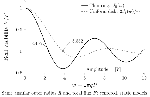
Signed real visibility $V/F$ for two ideal, centered, static circular brightness distributions with the same angular outer radius $R$ and flux $F$, where $w=2\pi qR$ and $q$ is baseline length in wavelengths. The curves are analytic Fourier transforms, with first zeros at $2.4048$ and $3.8317$. A negative lobe represents a phase reversal; an amplitude plot would show its absolute value. These models contain no black-hole geometry, scattering, noise, or reconstruction assumptions.

Closure quantities cancel station gains

Write $g_a=|g_a|e^{i\phi_a}$. Around a triangle of stations, the closure phase is

$$\psi_{abc}=\arg\!\left(V^{\rm obs}_{ab}V^{\rm obs}_{bc}V^{\rm obs}_{ca}\right).$$

The station phases enter as $(\phi_a-\phi_b)+(\phi_b-\phi_c)+(\phi_c-\phi_a)=0$, so the result is independent of those phase errors when the measurement model is truly station based. For four stations, a closure amplitude can be formed as

$$C_{abcd}= \frac{|V^{\rm obs}_{ab}|\,|V^{\rm obs}_{cd}|} {|V^{\rm obs}_{ac}|\,|V^{\rm obs}_{bd}|},$$

which similarly cancels station amplitude gains. These quantities retain source-structure information while discarding some calibration information.

Closure is not immunity from every systematic. Baseline-based corruption, polarization leakage, bandpass errors, source evolution within an averaging interval, and low-signal phase statistics can all survive or bias it. Redundant closure quantities are correlated rather than independent; high-signal Gaussian error propagation is inadequate when a denominator amplitude approaches zero. Blackburn and collaborators derive nonredundant closure sets and their covariance in Blackburn et al. 2020, §§ 2–4 and Appendices B–C.

A named M87* data release

The reproducible observational anchor is EHT data product 2019-D01-01, “First M87 EHT Results: Calibrated Data,” DOI 10.25739/g85n-f134. It contains calibrated Stokes-$I$ visibility products in low and high bands centered at 227.1 and 229.1 GHz for 2017 April 5, 6, 10, and 11, together with flags and station metadata. The 2017 array involved ALMA, APEX, the Large Millimeter Telescope, the IRAM 30-m telescope at Pico Veleta, the Submillimeter Telescope, the South Pole Telescope, the Submillimeter Array, and the James Clerk Maxwell Telescope; the South Pole Telescope could not observe M87*. M87* was observed on April 5, 6, and 11, with calibration scans on April 10.

The data reduction used HOPS as the primary fringe-fitting path and compared it with two independent paths: CASA-based rPICARD and AIPS. A priori amplitude calibration and network calibration used the colocated ALMA–APEX and SMA–JCMT baselines, while documented station-specific issues included LMT gain variation, a Pico Veleta clock problem, APEX gaps, and SMA/JCMT sideband contamination. Paper III gives the three pipelines separately in Event Horizon Telescope Collaboration 2019, §§ 5.1–5.3; its §§ 6–8 describe amplitude calibration, network calibration, and validation.

This release boundary matters. The public product is scan-averaged calibrated Stokes $I$; it is not raw voltage data, and it differs slightly from the parallel-hand RR/LL working data described in the 2019 imaging analysis. A reproduction must use the release flags rather than silently resurrecting excluded samples and must report station, day, band, coherent-averaging interval, and signal-to-noise selections.

Calibration, likelihood, and angular scale

A direct visibility analysis compares a forward model $V(\boldsymbol{\eta})$ with the sampled data, often through a complex-visibility or closure likelihood. The parameter vector $\boldsymbol{\eta}$ may include size, flux, orientation, asymmetry, and nuisance gains. Priors on gain stability, compact flux, positivity, or morphology are part of the inference and can change a credible interval. Treating every closure quantity as independent would count correlated information more than once; one must instead use a nonredundant set or its covariance.

Thermal noise supplies a statistical uncertainty conditional on the likelihood. Calibration errors, residual nonclosing terms, finite bandwidth and time averaging, refractive scattering, intrinsic variability, and source-model mismatch are systematic uncertainty or model dependence. They do not generally shrink by adding redundant closure triangles. Completeness also has a precise meaning here: the sampled $(u,v)$ plane is incomplete, and a detection threshold or flag can remove low-amplitude measurements in a structure-dependent way.

An angular feature becomes a physical scale only after external mass and distance information, an emission model, and the distinction between emission-ring diameter and metric critical-curve diameter are supplied. The EHT analysis used both visibility-domain features and multiple reconstruction/model families; its mass inference explicitly propagated calibration and model-library effects Event Horizon Telescope Collaboration 2019, §§ 3–6 and § 8. The measurement therefore constrains a model-conditioned angular scale, not the horizon surface directly.

Reproducing the analysis and interpreting its limits

As of the observational evidence cutoff 2026-08-18, a defensible teaching reproduction is:

1. obtain data product 2019-D01-01 from its DOI landing page and retain its release notes, flags, station names, dates, and two bands;
2. verify the point-source and circular-Gaussian Fourier transforms above on the exact released $(u,v)$ coordinates;
3. compute triangle closure phases and quadrangle log closure amplitudes, retaining their covariance and recording every signal-to-noise or flag selection;
4. inject arbitrary station gains into a synthetic visibility set and confirm that closures remain fixed while individual visibility phases and amplitudes change; and
5. fit at least one simple geometric model in visibility space, repeat it by day and band, and compare the inferred scale with and without the longest baselines.

This is an executable analysis specification, not a claim that this page reran the EHT pipelines. The release supplies calibrated data rather than every upstream raw-data calibration choice. A faithful research reproduction must also preserve software versions, random seeds, likelihood normalization, gain priors, and machine-readable outputs.

Common pitfalls

A long baseline is not a complete image. It sets access to fine Fourier structure along one direction. Sparse coverage can leave distinct images with nearly identical sampled visibilities.

Closure data are not calibration free. They cancel ideal station-based gains, not baseline errors, leakage, source evolution, or biased low-signal statistics.

A dark reconstruction is not a horizon detection by inspection. The chain from visibility to metric scale passes through calibration, inverse-problem assumptions, emitting-plasma physics, mass, and distance.

Exercises

Three stations have true baseline phases $\varphi_{AB}=20^\circ$, $\varphi_{BC}=-35^\circ$, and $\varphi_{CA}=50^\circ$. Their station phase errors are $\phi_A=40^\circ$, $\phi_B=-15^\circ$, and $\phi_C=25^\circ$. Find the observed baseline phases and show explicitly what the closure phase recovers.

Solution

The measurement equation adds $\phi_a-\phi_b$ to the true phase. Therefore

$$\begin{aligned} \varphi^{\rm obs}_{AB}&=20^\circ+40^\circ-(-15^\circ)=75^\circ,\\ \varphi^{\rm obs}_{BC}&=-35^\circ-15^\circ-25^\circ=-75^\circ,\\ \varphi^{\rm obs}_{CA}&=50^\circ+25^\circ-40^\circ=35^\circ. \end{aligned}$$

Their sum is $75^\circ-75^\circ+35^\circ=35^\circ$ modulo $360^\circ$. The true closure phase is also $20^\circ-35^\circ+50^\circ=35^\circ$. The individual observed phases are badly shifted, but the station terms telescope to zero. A baseline-based phase error would not cancel and is the discriminating failure case.

A second exercise: the same null, different radii

A circular source has its first visibility null at $q_1=4.0\times10^9$ wavelengths. Infer its angular radius under the thin-ring and uniform-disk models. How large is the modeling difference?

Solution

Using $1\ {\rm rad}=2.06265\times10^{11}\,\mu{\rm as}$,

$$\begin{aligned} R_{\rm ring}&=\frac{2.4048}{2\pi q_1} \simeq19.7\,\mu{\rm as},\\ R_{\rm disk}&=\frac{3.8317}{2\pi q_1} \simeq31.4\,\mu{\rm as}. \end{aligned}$$

The disk radius is about $59\%$ larger. These models need not fit the rest of the visibility data equally well; the exercise deliberately uses only one null. It shows why a precise null position can still leave a substantial morphology-dependent size uncertainty.

References

• Blackburn, Lindy, Dominic W. Pesce, Michael D. Johnson, et al. “Closure Statistics in Interferometric Data.” The Astrophysical Journal 894 (2020): 31. DOI.
• Event Horizon Telescope Collaboration. “First M87 EHT Results: Calibrated Data.” Data product 2019-D01-01 (2019). DOI.
• Event Horizon Telescope Collaboration. “First M87 Event Horizon Telescope Results. III. Data Processing and Calibration.” The Astrophysical Journal Letters 875 (2019): L3. DOI.
• Event Horizon Telescope Collaboration. “First M87 Event Horizon Telescope Results. VI. The Shadow and Mass of the Central Black Hole.” The Astrophysical Journal Letters 875 (2019): L6. DOI.
• Thompson, A. Richard, James M. Moran, and George W. Swenson Jr. Interferometry and Synthesis in Radio Astronomy. 3rd ed. Cham: Springer, 2017. DOI.