Near-Horizon Scaling Limits

Every smooth degenerate Killing horizon admits a canonical scaling that keeps the horizon at finite scaled transverse null coordinate while discarding positive-order transverse Taylor coefficients and retaining their horizon values. The limit is an exact spacetime geometry, not merely the first terms of a local approximation. It retains a metric, a one-form, and a function on one horizon cross-section, acquires a dilation symmetry, and forgets the asymptotic normalization of the parent black hole.

Helpful background. Exact Solutions of Einstein’s Equations supplies extremal Reissner–Nordström and Kerr examples; Causality and Global Structure supplies the distinction between a local limit and a global event horizon; The Einstein Equation supplies the reduced horizon equations; Black-Hole Perturbation Theory treats fields evolving on the limiting background; Black-Hole Geometry and Mechanics supplies degenerate Killing horizons and Gaussian-null coordinates.

The scaling term by term

Near a smooth degenerate Killing horizon, choose Gaussian-null coordinates $(v,r,x^A)$ in which the horizon is $r=0$ and its normal Killing field is $K=\partial_v$. The metric is

$$ds^2=2\,dv\!\left(dr+r h_A(r,x)dx^A +\frac12r^2F(r,x)dv\right)+\gamma_{AB}(r,x)dx^A dx^B.$$

For $\varepsilon\gt0$, pull the metric back by

$$v_{\rm old}=\frac{v}{\varepsilon}, \qquad r_{\rm old}=\varepsilon r, \qquad x^A_{\rm old}=x^A.$$

For each $\varepsilon\gt0$, this is a diffeomorphism of the Gaussian-null coordinate patch. The limit is evaluated at fixed new coordinates: fixed $r=R$ means $r_{\rm old}=\varepsilon R\to0$, whereas a fixed point inside the parent Gaussian-null patch, $r_{\rm old}=\rho_*\gt0$, appears at $r=\rho_*/\varepsilon\to\infty$. There is no $\varepsilon=0$ coordinate transformation.

The four kinds of terms transform separately:

$$\begin{aligned} 2\,dv_{\rm old}dr_{\rm old}&=2\,dv\,dr,\\ 2r_{\rm old}h_A(r_{\rm old},x)dv_{\rm old}dx^A &=2r h_A(\varepsilon r,x)dv\,dx^A,\\ r_{\rm old}^2F(r_{\rm old},x)dv_{\rm old}^2 &=r^2F(\varepsilon r,x)dv^2,\\ \gamma_{AB}(r_{\rm old},x)dx^A dx^B &=\gamma_{AB}(\varepsilon r,x)dx^A dx^B. \end{aligned}$$

Smoothness now makes the limit immediate:

$$ds^2_{\rm NH}=2\,dv\!\left(dr+r h_A(x)dx^A +\frac12r^2F(x)dv\right)+\gamma_{AB}(x)dx^A dx^B.$$

Here $F(x)=F(0,x)$, $h_A(x)=h_A(0,x)$, and $\gamma_{AB}(x)=\gamma_{AB}(0,x)$. The triple $(F,h_A,\gamma_{AB})$ is the near-horizon data. The construction and the existence statement are Kunduri and Lucietti 2013, §2.1, pp. 11–12, Eqs. (6)–(7).

This convergence is on bounded regions of the scaled coordinates; it does not choose a global completion of the limiting spacetime. The figure follows one bounded scaled window back to its shrinking parent neighborhood and tracks a fixed point in the local parent patch in the opposite direction. The asymptotic region is outside this local construction and is not inherited by the limit.

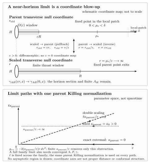
For every $\varepsilon\gt0$, $v_{\rm old}=v/\varepsilon$ and $r_{\rm old}=\varepsilon r$ merely pull the parent metric back to new coordinates. A bounded scaled interval $0\leq r\leq R$ samples the shrinking parent band $0\leq r_{\rm old}\leq\varepsilon R$, while a fixed point $r_{\rm old}=\rho_*$ inside the local Gaussian-null patch moves to $r=\rho_*/\varepsilon$ and leaves every bounded scaled chart. The horizon remains at $r=0$; its cross-section metric and, when finite, its area survive. The parent asymptotic completion lies outside this local construction and is not inherited. With one parent Killing normalization, the inset distinguishes the exact-extremal path $\kappa_{\rm parent}=0$ from fixed positive surface gravity and the dimensionless correlated path $\ell\kappa_{\rm parent}/\varepsilon\to\alpha$ for fixed $\ell$. A finite correlated metric also requires convergence of the remaining horizon data. This is a schematic coordinate map, not a proper-distance enlargement or conformal diagram, and is not to scale.

Why degeneracy is essential

For a nondegenerate Killing horizon, $g_{vv}$ begins as $-2\kappa r+O(r^2)$. Under the same scaling its leading contribution becomes $-2\kappa r\,dv^2/\varepsilon$, which diverges. A finite limit would require a different operation, such as also changing a family parameter or rescaling the metric. It would no longer be the intrinsic near-horizon limit of one fixed spacetime.

The degenerate limit has an exact isometry

$$v\longmapsto\frac{v}{c}, \qquad r\longmapsto cr,$$

generated by $D=-v\partial_v+r\partial_r$. Together with $K=\partial_v$, it obeys $[D,K]=K$. The parent spacetime need not possess this dilation: it emerges because every positive power of $r$ beyond the displayed near-horizon data has been scaled away.

Field equations become equations on the cross-section

For every positive $\varepsilon$, the pulled-back metric is diffeomorphic to the parent metric. If the fields and their derivatives converge smoothly, diffeomorphism-covariant local field equations pass to the limit. In vacuum Einstein gravity with cosmological constant $\Lambda$, the independent equations reduce to

$$R_{AB}(\gamma)=\frac12h_Ah_B-\nabla_{(A}h_{B)} +\Lambda\gamma_{AB},$$

and

$$F=\frac12h_Ah^A-\frac12\nabla_Ah^A+\Lambda.$$

All derivatives here use the Riemannian cross-section metric $\gamma$. The remaining spacetime Einstein equations follow from these and the Bianchi identity. With matter, additional horizon fields and equations appear; it is not automatic that an arbitrary nonsmooth potential has a limit even when its stress tensor does. The precise reduction, including Maxwell fields, is in Kunduri and Lucietti 2013, §2.3, pp. 13–15, Eqs. (15)–(29).

This reduction is powerful but asymmetric. Every smooth degenerate solution produces near-horizon data satisfying the reduced equations. A solution of the reduced equations need not extend to a complete black hole with the desired asymptotics.

For a smooth invariant Maxwell two-form, the same scaling has the general finite form

$$\mathcal F_{\rm NH} =d\!\left(r\Delta(x)dv\right) +\frac12B_{AB}(x)dx^A\wedge dx^B,$$

where $B$ is closed on $H$. The first term contains the horizon electric data and the second the magnetic data intrinsic to the cross-section. Smoothness and the horizon constraint eliminate a potentially divergent $dv\wedge dx^A$ term. This example shows why one must scale every matter field, not merely insert the limiting metric into its stress tensor after the fact.

Near-horizon and near-extremal limits differ

The operation above keeps one exactly degenerate spacetime fixed and sends $\varepsilon$ to zero. A near-extremal limit instead changes a family parameter so that $\kappa\to0$. The operations need not commute. At fixed positive $\kappa$, the linear contribution $g_{vv}=-2\kappa r+O(r^2)$ diverges under the degenerate scaling. A joint limit can remain finite only after choosing a common normalization of the parent Killing generator, requiring $\kappa/\varepsilon\to\widehat\kappa$, and requiring the remaining Gaussian-null data to converge smoothly. Boundedness expressed only as $\kappa=O(\varepsilon)$ is insufficient to select a unique limit.

In the Kerr family, the exactly extremal throat is the near-horizon extreme Kerr (NHEK) geometry. A correlated double scaling may instead produce its finite-temperature near-NHEK form, but the extra constant records how the two limits were correlated. This scaling is developed in Bredberg et al. 2010, §3, pp. 6–8, Eqs. (3.1)–(3.9). It is not part of the intrinsic data of the exactly degenerate horizon. Therefore three geometries must be kept distinct: the full near-extremal exterior, the exact extremal exterior, and the exact extremal near-horizon geometry. They can have different global boundaries and different preferred time normalizations.

The Near-Horizon Extreme Kerr Geometry page derives the exactly extremal NHEK metric and its enhanced symmetry.

There is residual coordinate freedom even in the exact limit. A constant rescaling of $v$ accompanied by the inverse rescaling of $r$ is an isometry of the limiting metric, and diffeomorphisms of $H$ relabel the cross-section data. Consequently a classification concerns equivalence classes of $(F,h,\gamma)$, not raw coordinate components. Dimensionless curvature, topology, charges expressible as horizon integrals, and regularity at fixed points of rotational symmetries provide better comparisons than a component- by-component match.

What the limit retains and what it loses

The cross-section metric retains the horizon area whenever that area is finite, in particular for a compact cross-section. With rotational symmetry and suitable field equations, angular momentum and gauge charges can also be written as horizon integrals. The mass and the horizon angular velocity relative to infinity cannot: the scaling sends the asymptotic region out of the limiting spacetime and introduces a freedom to rescale $v$. This loss is spelled out in Kunduri and Lucietti 2013, §2.4, pp. 15–16.

Accordingly, $ds^2_{\rm NH}$ is not a globally magnified subset of the original Penrose diagram. A fixed value of the new $r$ corresponds to $r_{\rm old}=\varepsilon r$, ever closer to the horizon. The limiting geometry can be geodesically extended into regions for which no point remains at fixed coordinates in the parent exterior. It records universal throat structure, not the full global completion.

Solved diagnostic: the charged static throat

Let $L=GM$ and begin with extremal Reissner–Nordström in ingoing coordinates, using $\rho=R-L$:

$$ds^2=-\frac{\rho^2}{(L+\rho)^2}dv_{\rm old}^2 +2\,dv_{\rm old}d\rho+(L+\rho)^2d\Omega_2^2.$$

Set $v_{\rm old}=v/\varepsilon$ and $\rho=\varepsilon r$. Find the limit and give two independent checks.

Solution

Substitution gives

$$ds^2_\varepsilon=-\frac{r^2}{(L+\varepsilon r)^2}dv^2 +2\,dv\,dr+(L+\varepsilon r)^2d\Omega_2^2,$$

so

$$ds^2_{\rm NH}=-\frac{r^2}{L^2}dv^2+2\,dv\,dr +L^2d\Omega_2^2.$$

This is $\mathrm{AdS}_2\times S^2$ in an ingoing Poincaré patch, with equal radii $L$. First, it is invariant under $v\mapsto v/c$, $r\mapsto cr$. Second, its factor curvatures are $R_{\mathrm{AdS}_2}=-2/L^2$ and $R_{S^2}=2/L^2$, so the four-dimensional scalar curvature vanishes, as required by the trace-free Maxwell stress tensor. The asymptotically flat region has disappeared even though the horizon two-sphere and its area remain.

The next page applies the same operation to obtain the near-horizon extreme Kerr geometry. Classification then asks which triples $(F,h,\gamma)$ solve the reduced equations, not which full black holes have already been constructed.

References

• Bredberg, Irene, Thomas Hartman, Wei Song, and Andrew Strominger. “Black Hole Superradiance From Kerr/CFT.” Journal of High Energy Physics 2010, 019 (2010). DOI. Open PDF.
• Kunduri, Hari K., and James Lucietti. “Classification of Near-Horizon Geometries of Extremal Black Holes.” Living Reviews in Relativity 16, 8 (2013). DOI.