Scalar and Electromagnetic Perturbations of Schwarzschild

Scalar and electromagnetic waves travel on the same Schwarzschild geometry, but spherical reduction gives them different radial barriers. A massless scalar retains a curvature term even in its monopole; Maxwell’s two radiative parities share a simpler potential and have no propagating monopole. We derive these statements, reconstruct the electromagnetic field, and connect the radial Wronskian to measured energy flow. The background is fixed and four dimensional: the scalar is neutral and minimally coupled, Maxwell’s equations are source free, and metric backreaction is excluded.

Required background. PDEs and Green Functions for Gravitation supplies separation of variables, conserved Wronskians, and characteristic boundary conditions.

Helpful background. Black-Hole Geometry and Mechanics fixes the horizon and asymptotic regions; Formulations of General Relativity distinguishes Maxwell gauge constraints from evolution; Killing Fields and Isometry Groups explains the conserved frequency and angular labels.

Schwarzschild metric

Let $\mu=GM\gt0$ be the Schwarzschild mass length, not a field mass:

$$ds^2=-f\,dt^2+f^{-1}\,dr^2+r^2\,d\Omega^2, \qquad f=1-\frac{2\mu}{r}, \qquad r\gt2\mu.$$

Use the tortoise coordinate $x=r_*$ with its additive constant fixed here by

$$x=r+2\mu\ln\left(\frac{r}{2\mu}-1\right), \qquad \partial_x=f\partial_r.$$

Thus the horizon and spatial infinity lie at $x\to-\infty$ and $x\to+\infty$. A different additive constant shifts phases and the horizontal origin of a potential plot, but not energy fluxes.

It suffices to work with one real, unit-normalized spherical harmonic $Y$. Write $L=\ell(\ell+1)$ and let $D_A$, $\Omega_{AB}$ and $\epsilon_{AB}$ be the derivative, metric and orientation tensor of the unit sphere:

$$D^2Y=-LY,\qquad \int_{S^2}Y^2\,d\Omega=1, \qquad \epsilon_{\theta\phi}=\sin\theta.$$

Real sine/cosine combinations of the usual complex harmonics give such a basis; linear superposition restores a general real field. For $\ell\ge1$, define the axial vector as in Tensor Harmonics and Parity Decomposition:

$$X_A=-\epsilon_A{}^B D_BY,\qquad D_AX_B-D_BX_A=-L\epsilon_{AB}Y,$$ $$\int_{S^2}D_AYD^AY\,d\Omega =\int_{S^2}X_AX^A\,d\Omega=L.$$

Angular indices in these identities are raised with $\Omega^{AB}$, not the four-dimensional angular inverse metric $r^{-2}\Omega^{AB}$. The Maxwell test-field page uses the opposite sign for $X_A$. For the same physical odd field, $X_A^{\mathrm{here}}=-X_A^{\mathrm{Maxwell}}$ and $\Psi_-^{\mathrm{here}}=-\Psi_-^{\mathrm{Maxwell}}$; the even amplitude does not change.

The scalar curvature barrier

For a real scalar with action

$$S_0=-\frac12\int \nabla_\mu\Phi\nabla^\mu\Phi\sqrt{-g}\,d^4x, \qquad \Phi=\frac{\psi_0(t,r)}rY,$$

the field equation is $\Box\Phi=0$. Its full coordinate form is

$$\Box\Phi=-\frac1f\partial_t^2\Phi +\frac1{r^2}\partial_r\!\left(r^2f\partial_r\Phi\right) +\frac1{r^2}D^2\Phi.$$

The useful cancellation is not merely the angular eigenvalue. Differentiating the factor $1/r$ gives the radial identity

$$fr\left[\frac1{r^2}\partial_r\!\left( r^2f\partial_r\frac{\psi_0}{r}\right)\right] =\partial_x^2\psi_0-\frac{ff'}r\psi_0, \qquad f'=\frac{df}{dr}.$$

Multiplying the full field equation by $rf$ therefore yields

$$\left[-\partial_t^2+\partial_x^2-V_0(r)\right]\psi_0=0, \qquad V_0=f\left(\frac{L}{r^2}+\frac{2\mu}{r^3}\right).$$

The extra term is a consequence of the curved radial geometry and the area rescaling, not an added mass or a nonminimal coupling. The covariant equation and stress tensor follow from the massless specialization of Wald 1984, §4.3, p. 70, Eqs. (4.3.9)–(4.3.10). The derivation above fixes the particular radial normalization used here.

Maxwell radiation in two parity sectors

Choose the canonical real-field Maxwell action, writing $F=dA$ locally:

$$S_1=-\frac14\int F_{\mu\nu}F^{\mu\nu}\sqrt{-g}\,d^4x.$$

Its equations are $\nabla_\mu F^{\mu\nu}=0$ and $dF=0$. This action has no $1/(4\pi)$ multiplier: its stress tensor is $4\pi$ times Wald’s Gaussian-unit tensor for the same numerical $F$. The source-free equations are unchanged. Wald 1984, §4.3, p. 70, Eqs. (4.3.12)–(4.3.14)

Odd radiation and the electric invariant

For this subsection take $\ell\ge1$ and orbit indices $a=t,r$. In odd parity, set $A_a=0$ and $A_A=\Psi_-X_A$. The angular Maxwell equation directly gives

$$-\frac1f\partial_t^2\Psi_-+ \partial_r(f\partial_r\Psi_-)-\frac{L}{r^2}\Psi_-=0.$$

In even parity write $A_a=a_aY$, $A_A=bD_AY$. A gauge transformation with parameter $\lambda(t,r)Y$ sends $a_a$ to $a_a+\partial_a\lambda$ and $b$ to $b+\lambda$. Thus

$$p_a=a_a-\partial_ab,\qquad e=\partial_tp_r-\partial_rp_t,\qquad F_{tr}=eY,\qquad F_{aA}=-p_aD_AY$$

are gauge invariant. The $t$ and $r$ Maxwell equations become

$$\partial_r(r^2e)+\frac{L}{f}p_t=0, \qquad -\partial_t(r^2e)-Lf p_r=0.$$

Define the electric master amplitude and solve these equations:

$$\Psi_+=\frac{r^2e}{L},\qquad p_t=-f\partial_r\Psi_+,\qquad p_r=-\frac1f\partial_t\Psi_+.$$

Substitution into the definition of $e$ gives the same radial equation as in odd parity. The remaining angular Maxwell equation is

$$\frac1f\partial_tp_t-\partial_r(fp_r)=0;$$

after reconstruction it is the equality of mixed partial derivatives. Consequently each parity satisfies

$$\left[-\partial_t^2+\partial_x^2-V_1(r)\right]\Psi_\pm=0, \qquad V_1=f\frac{L}{r^2},\qquad \ell\ge1.$$

The classical Maxwell radial reduction also appears in Price 1972, §III.D.1, p. 2445, Eqs. (45a)–(45b), PDF. That formula supports the spin-one potential, not the scalar curvature term derived separately above.

Reconstructing the physical field

For a solution of either master equation, all independent components are:

Component	Odd parity	Even parity
$F_{tr}$	$0$	$L\Psi_+Y/r^2$
$F_{tA}$	$(\partial_t\Psi_-)X_A$	$f(\partial_r\Psi_+)D_AY$
$F_{rA}$	$(\partial_r\Psi_-)X_A$	$f^{-1}(\partial_t\Psi_+)D_AY$
$F_{AB}$	$-L\Psi_-\epsilon_{AB}Y$	$0$

The two potentials coincide, but the field components do not. Conversely, an even master solution gives a source-free field because the orbit Maxwell equations hold identically, while its Bianchi identity is precisely the master equation. No extra electromagnetic gauge condition is needed to recover $F$.

Apparent factors $f^{-1}$ must be assessed in regular coordinates. Set $v=t+x$. Transforming the even two-form, rather than just substituting a radial limit into its Schwarzschild components, gives

$$F_{rA}^{(v,r)}=F_{rA}^{(t,r)}-f^{-1}F_{tA}^{(t,r)} =-(\partial_r\Psi_+)_vD_AY.$$

For odd parity the corresponding component is $F_{rA}^{(v,r)}=(\partial_r\Psi_-)_vX_A$. Smooth master fields in $(v,r)$ therefore have smooth reconstructed components at the future horizon.

Comparing the radial barriers

Both potentials have dimensions of inverse length squared, are nonnegative in the exterior, and tend to zero at both ends of the tortoise line. At the same allowed multipole their difference is particularly simple:

$$V_0-V_1=\frac{2\mu f}{r^3}\gt0\qquad(r\gt2\mu).$$

The following dipole comparison uses $\ell=1$, the lowest common radiative multipole. Inspect both the height and the position of each maximum. Since $dr/dx=f\gt0$ in the exterior, finding an extremum with respect to $r$ also locates the extremum with respect to $x$.

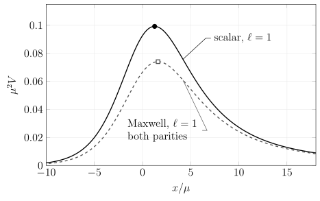
At $\ell=1$ the scalar barrier is higher than the common Maxwell barrier and peaks slightly closer to the horizon. The quantitative curves use $\mu=GM$ and the displayed tortoise coordinate with zero additive constant. This finite window does not reach either asymptotic zero; barrier height alone does not determine reflection or a quasinormal frequency.

Dipole field	Peak radius $r/\mu$	Peak coordinate $x/\mu$	Peak height $\mu^2V$
Scalar	$(3+\sqrt{73})/4\simeq2.886001$	$1.257632$	$0.099262$
Either Maxwell parity	$3$	$1.613706$	$2/27\simeq0.074074$

The scalar barrier is higher and peaks slightly closer to the horizon. This geometric comparison does not determine a reflection coefficient or a quasinormal frequency: those require solving a specified boundary problem. Far from the hole both potentials have leading centrifugal term $L/r^2$ when $L\gt0$; the scalar monopole instead starts at order $r^{-3}$.

Physical energy and positive-frequency scattering

The conserved radial Wronskian is not automatically a physical power with unit coefficient. The canonical actions fix the stresses

$$\begin{aligned} T^{(0)}_{\mu\nu} &=\nabla_\mu\Phi\nabla_\nu\Phi -\tfrac12g_{\mu\nu}\nabla_\alpha\Phi\nabla^\alpha\Phi,\\ T^{(1)}_{\mu\nu} &=F_{\mu\alpha}F_\nu{}^\alpha -\tfrac14g_{\mu\nu}F_{\alpha\beta}F^{\alpha\beta}. \end{aligned}$$

Outward power associated with the Killing field $\partial_t$ is $P=-r^2\int_{S^2}T^r{}_t\,d\Omega$. Inserting the scalar field and the reconstruction table and using the angular norms gives, for one real mode,

$$\begin{aligned} P_0&=-(\partial_t\psi_0) \left(\partial_x\psi_0-\frac fr\psi_0\right)\\ &=-(\partial_t\psi_0)(\partial_x\psi_0) +\frac12\partial_t\!\left(\frac fr\psi_0^2\right),\\ P_1&=-L(\partial_t\Psi_\pm)(\partial_x\Psi_\pm). \end{aligned}$$

The scalar’s finite-radius correction is a total time derivative, not an instantaneously vanishing term. The factor $L$ in Maxwell power comes from the derivative harmonic’s norm, not a different group velocity. Equal scalar and Maxwell master amplitudes need not carry equal power.

Now restrict to real $\omega\gt0$ and use a real physical master field $\psi(t,x)=\operatorname{Re}[u(x)e^{-i\omega t}]$, where $\psi$ denotes $\psi_0$ or $\Psi_\pm$. Then

$$u''+(\omega^2-V_s)u=0,\qquad \mathcal J=\frac{\overline u u'-u\overline u'}{2i}, \qquad u'=\frac{du}{dx}.$$

The radial equation implies $\mathcal J'=0$. Averaging over the physical period $2\pi/\omega$ gives

$$\langle P_0\rangle=\frac\omega2\mathcal J, \qquad \langle P_1\rangle=\frac{L\omega}{2}\mathcal J.$$

The factor $1/2$ is the cycle average of a real sinusoid; the scalar total derivative has zero cycle average. For a wave incident from infinity, normalize each sector separately by

$$u\sim \begin{cases} T e^{-i\omega x},&x\to-\infty,\\ e^{-i\omega x}+R e^{+i\omega x},&x\to+\infty. \end{cases}$$

At the future horizon the ingoing full mode has leading dependence $e^{-i\omega v}$ with a regular radial factor. Its oscillation in $v$ is physical; the singularity of Schwarzschild time is the coordinate effect. The potential is only asymptotically zero, so an arbitrary function of $v$ alone is not an exact finite-radius solution. Nor does smoothness alone select the usual boundary branch for every complex frequency.

Evaluating the current at both ends gives

$$\mathcal J_\infty=\omega(|R|^2-1),\qquad \mathcal J_H=-\omega|T|^2,\qquad 1-|R|^2=|T|^2.$$

Negative outward horizon power means positive energy entering the hole. There is no superradiant amplification for these neutral fields on a static Schwarzschild background. The normalization factors cancel within each sector’s power ratio. At zero frequency the two traveling-wave bases degenerate; for complex frequency there is no real cycle average and the current generally is not constant. Neither case inherits this scattering argument unchanged.

Scalar monopoles and conserved Maxwell charges

The scalar reduction remains valid at $\ell=0$:

$$\left[-\partial_t^2+\partial_x^2- \frac{2\mu f}{r^3}\right]\psi_0=0.$$

Spherical scalar waves are dynamical despite having no angular momentum. For Maxwell theory, however, both $D_AY$ and $X_A$ vanish at $\ell=0$ and the definition of $\Psi_+$ would divide by zero. Solve that sector directly. The general spherically symmetric field strength is

$$F=\frac{C_E(t,r)}{r^2}\,dt\wedge dr +C_B(t,r)\sin\theta\,d\theta\wedge d\phi.$$

The two orbit Maxwell equations and the Bianchi identity respectively give

$$\partial_rC_E=0,\qquad\partial_tC_E=0, \qquad\partial_rC_B=0,\qquad\partial_tC_B=0.$$

Thus $C_E$ and $C_B$ are constant electric and magnetic Coulomb coefficients, not radiative amplitudes. Radial Gauss law alone would permit $C_E=Q(t)$; the second equation is essential to establish conservation in time. The magnetic surface flux is $\int_{S^2}F=4\pi C_B$. Requiring a single globally smooth potential on the sphere excludes nonzero $C_B$ by Stokes’ theorem; local source-free Maxwell theory itself does not exclude it.

Radiation therefore starts at $\ell=0$ for the scalar and at $\ell=1$ for Maxwell. A zero curve obtained by putting $L=0$ in $V_1$ would not represent a missing Maxwell radiative mode. With background $F=0$, electromagnetic stress is quadratic in the small field, so a linear Coulomb field does not produce a first-order Reissner–Nordström metric correction. Coupled perturbations about a background with nonzero charge belong to Charged Spherical Black Holes and Coupled Sectors.

Exercises

Locate the dipole maxima

Set $\rho=r/\mu\gt2$. Derive the two peak radii in the table and check that they are maxima. Does a higher barrier alone prove stronger reflection at every frequency?

Solution

The dimensionless dipole potentials and their derivatives are

$$\begin{aligned} \mu^2V_0&=\frac{2(\rho-2)(\rho+1)}{\rho^4},& \frac{d(\mu^2V_0)}{d\rho} &=-\frac{2(2\rho^2-3\rho-8)}{\rho^5},\\ \mu^2V_1&=\frac{2(\rho-2)}{\rho^3},& \frac{d(\mu^2V_1)}{d\rho} &=-\frac{4(\rho-3)}{\rho^4}. \end{aligned}$$

Only $\rho_0=(3+\sqrt{73})/4$ and $\rho_1=3$ lie in the exterior. At these roots the second derivatives are respectively $-2(4\rho_0-3)/\rho_0^5\lt0$ and $-4/81\lt0$. Substitution into $x/\mu=\rho+2\ln(\rho/2-1)$ gives the plotted positions. Barrier height alone is not a scattering calculation; the full shape, frequency and boundary conditions enter the wave equation.

Find the missing monopole equation

Consider $F=Q(t)r^{-2}dt\wedge dr$. Verify that it obeys the radial Gauss constraint and $dF=0$ for arbitrary differentiable $Q$. Which remaining equation rules out a varying vacuum charge?

Solution

The inverse metric gives $F^{rt}=Q(t)/r^2$. Therefore $\nabla_\mu F^{\mu t}=r^{-2}\partial_r(r^2F^{rt})=0$, and differentiating the two-form gives $dF=0$ because every term repeats $dt$ or $dr$. But

$$\nabla_\mu F^{\mu r} =\frac1{r^2}\partial_t(r^2F^{tr}) =-\frac{Q'(t)}{r^2}.$$

Vacuum Maxwell theory therefore requires $Q'=0$. A varying coefficient would need a radial electric current; satisfying an initial constraint is not the same as satisfying the evolution equations.

Check the scalar power correction

At a fixed exterior radius $r_0$, suppose the scalar master amplitude has trace $\psi_0(t,r_0)=A\cos(\omega t)$ with real $A$ and $\omega\gt0$. Find the difference between physical power and $-\psi_{0,t}\psi_{0,x}$, and its cycle average.

Solution

The correction is

$$\frac12\partial_t\!\left(\frac{f(r_0)}{r_0}\psi_0^2\right) =-\frac{f(r_0)A^2\omega}{2r_0}\sin(2\omega t).$$

It is generally nonzero instantaneously but averages to zero over a period. The prescribed trace determines this correction only: without the radial derivative it does not specify the complete power, nor does it construct a solution of the field equation.

References

• Price, Richard H. “Nonspherical Perturbations of Relativistic Gravitational Collapse. II. Integer-Spin, Zero-Rest-Mass Fields.” Physical Review D 5 (1972): 2439–2454. DOI. Open PDF.
• Wald, Robert M. General Relativity. Chicago: University of Chicago Press, 1984. Publisher.