Reaction Rates, Decoupling, and Freeze-Out

Freeze-out is a loss of tracking, not an event that occurs at an infinitely sharp temperature. An interaction maintains equilibrium only when its relaxation rate is fast compared with the rate at which the expanding background moves the equilibrium state. The familiar estimate $\Gamma\sim H$ is therefore a useful scale locator, but the Boltzmann equation determines how gradual the departure is and what abundance or momentum distribution survives.

Required background. States, Processes, and the Laws of Thermodynamics supplies Thermodynamics and Statistical Mechanics for equilibrium, temperature, entropy, and chemical work.

Helpful background. The Einstein Equation supplies the Einstein-equation convention, while The Friedmann Equations supplies the cosmological $H$; Relativistic Matter and Compact Objects supplies Relativistic Matter and Compact Objects thermodynamics; Classical Field Modes and Canonical Variables supplies the Flat-Spacetime Quantum Field Theory mode convention; and Free Fields, Creation Operators, and Fock Space supplies occupation-state counting used in thermal collision terms.

Expansion and the collision term

Let $p$ be physical momentum and let $f_\chi(t,p)$ be the homogeneous, isotropic distribution of a species $\chi$. With the collision operator normalized to have units of inverse time, its Boltzmann equation is

$$\left(\frac{\partial}{\partial t} -Hp\frac{\partial}{\partial p}\right)f_\chi =\mathcal C_\chi[f].$$

The term $-Hp\partial_p f$ is cosmological redshifting. It is present even when $\mathcal C_\chi=0$, so “decoupled” does not mean “unchanging”: free momenta still scale as $a^{-1}$.

For a self-conjugate species annihilating through $\chi\chi\leftrightarrow a b$, suppose $a$ and $b$ remain in an equilibrium bath and Maxwell–Boltzmann number statistics are adequate. Closing the momentum-integrated equation also requires kinetic equilibrium for $\chi$:

$$f_\chi(t,p) =\frac{n_\chi(t)}{n_{\chi,\rm eq}(t)}f_{\chi,\rm eq}(t,p).$$

This ansatz allows the nonequilibrium normalization to factor out of the collision integral while the momentum shape remains thermal. Under these assumptions, integration over momentum gives

$$\boxed{ \dot n_\chi+3Hn_\chi =-\langle\sigma v_{\rm rel}\rangle \left(n_\chi^2-n_{\chi,\rm eq}^2\right) }.$$

The counting can be made explicit. For identical incoming particles, the annihilation event rate per physical volume is $R_{\rm ann}=\tfrac12\langle\sigma v_{\rm rel}\rangle n_\chi^2$; each event removes two $\chi$ particles, so the factors of two cancel and give the coefficient displayed above. For a distinct particle–antiparticle pair,

$$\begin{aligned} \dot n_\chi+3Hn_\chi &=-\langle\sigma v_{\rm rel}\rangle \left(n_\chi n_{\bar\chi} -n_{\chi,\rm eq}n_{\bar\chi,\rm eq}\right),\\ \dot n_{\bar\chi}+3Hn_{\bar\chi} &=-\langle\sigma v_{\rm rel}\rangle \left(n_\chi n_{\bar\chi} -n_{\chi,\rm eq}n_{\bar\chi,\rm eq}\right). \end{aligned}$$

If the population is charge symmetric, define $n_{\rm tot}=n_\chi+n_{\bar\chi}=2n_\chi$ and likewise in equilibrium. Summing the two equations gives

$$\dot n_{\rm tot}+3Hn_{\rm tot} =-\frac12\langle\sigma v_{\rm rel}\rangle \left(n_{\rm tot}^2-n_{{\rm tot},\rm eq}^2\right).$$

For an asymmetric population, the annihilation conserves $(n_\chi-n_{\bar\chi})a^3$, so one must evolve both densities or evolve the total density together with that conserved asymmetry. Once kinetic equilibrium also fails, the factorized closure above no longer follows; a momentum-dependent Boltzmann equation, or explicitly defined nonequilibrium averages, is needed.

The inverse term is not optional. Detailed balance makes the collision term vanish at equilibrium, and chemical equilibrium imposes $2\mu_\chi=\mu_a+\mu_b$. A phase-space derivation, including the closure and the identical-versus-distinct counting, is given in Gondolo and Gelmini 1991, §2, printed pp. 147–152, eqs. (2.4)–(2.24) (author-uploaded full text).

There is a source-level sign trap worth making explicit. Equation (27.2) of the 2026 Particle Data Group review prints $\dot n-3Hn$; the minus sign is a typographical error. The comoving-volume identity $a^{-3}d(a^3n)/dt=\dot n+3Hn$ fixes the plus sign used here. The surrounding discussion and the hot- and cold-relic limits are in PDG 2026, §27.3, printed pp. 2–4, eqs. (27.2)–(27.6) (Official PDF).

What the rate comparison actually tests

Near equilibrium, first factor out collisionless dilution and linearize a relevant observable $X$—for example the yield $n/s$ in an adiabatic bath, a temperature ratio, or a distortion amplitude—as

$$\frac{dX}{dt} =-\Gamma_{\rm rel}(X-X_{\rm eq}).$$

Writing $N=\ln a$ and $r=\Gamma_{\rm rel}/H$, the leading tracking error is

$$X-X_{\rm eq} \simeq-\frac{1}{r}\frac{dX_{\rm eq}}{dN}.$$

Thus equilibrium tracking requires more precisely

$$\Gamma_{\rm rel} \gg H\left|\frac{d\ln X_{\rm eq}}{d\ln a}\right|,$$

when $X_{\rm eq}$ is nonzero. The shorthand $\Gamma\gg H$ is adequate only when the equilibrium target changes by an order-one fraction per Hubble time. For a nonrelativistic equilibrium yield, the Boltzmann factor $e^{-m/T}$ can make the logarithmic derivative of order $x=m/T$, so the crossing $\Gamma=H$ is not an exact freeze-out surface. Moreover, $\Gamma_{\rm rel}$ is the relevant eigenvalue of the linearized collision operator; a large total scattering rate need not efficiently relax the particular mode of interest. For example, holding the bath target fixed and linearizing the self-conjugate number equation about equilibrium gives a collision term $-2n_{\chi,\rm eq}\langle\sigma v_{\rm rel}\rangle\delta n_\chi$. Thus its local number-relaxation rate is approximately $\Gamma_{\rm rel}=2n_{\chi,\rm eq}\langle\sigma v_{\rm rel}\rangle$, before allowing for coupled modes or changes in the thermal average.

The standard timescale comparison and its neutrino example are developed in PDG 2026, §22.3.3, printed pp. 12–13, eqs. (22.45)–(22.51) (Official PDF) and Tong 2019, §2.3.4, printed pp. 103–105 (Official PDF).

Chemical and kinetic decoupling

Different collision moments answer different physical questions.

Regime	Collision requirement	Consequence
Chemical equilibrium	Relevant number-changing reactions are rapid	The associated number-density combinations track their equilibrium values
Chemical freeze-out	Relevant number-changing reactions are too slow	Number density is no longer forced to its equilibrium value; a chemical potential or conserved yield develops
Kinetic equilibrium	Momentum and energy relaxation are rapid	The distribution shape and species temperature track the bath; chemical equilibrium is a separate question
Kinetic freeze-out	Momentum and energy relaxation are too slow	The distribution shape or species temperature no longer tracks the bath; number-changing reactions may be either effective or ineffective

Chemical decoupling is controlled by number-changing processes. After it, $n_\chi a^3$ can approach a constant even while elastic collisions keep $f_\chi$ close to a thermal shape at the bath temperature. Kinetic decoupling is controlled by momentum-transfer—not merely collision—rates; small-angle scatterings can be frequent yet transfer energy inefficiently. After kinetic decoupling, collisionless relativistic momenta redshift as $a^{-1}$, whereas the effective temperature of a nonrelativistic ideal gas redshifts as $a^{-2}$. Which decoupling occurs first is model-dependent, although chemical freeze-out followed by later kinetic decoupling is common for massive thermal relics.

Rate scaling and possible recoupling

Suppose relativistic targets have $n_{\rm targ}\propto T^3$ and $\langle\sigma v\rangle\propto T^q$. Distinguish the energy and entropy degrees of freedom by

$$\rho_r=\frac{\pi^2}{30}g_*T^4, \qquad s=\frac{2\pi^2}{45}g_{*s}T^3.$$

For an adiabatic bath, $g_{*s}T^3a^3$ is constant, so in general $T\propto g_{*s}^{-1/3}a^{-1}$. If both $g_*$ and $g_{*s}$ vary slowly during radiation domination, this reduces locally to $T\propto a^{-1}$ and

$$\begin{aligned} \Gamma\sim n_{\rm targ}\langle\sigma v\rangle &\propto T^{q+3},\\ H&=1.66\,g_*^{1/2}\frac{T^2}{M_{\rm Pl}}. \end{aligned}$$

Here $M_{\rm Pl}=G^{-1/2}\simeq1.22\times10^{19}\,{\rm GeV}$ is the nonreduced Planck mass. The coefficient $1.66$ belongs to this convention; it must not be paired with the reduced Planck mass $\bar M_{\rm Pl}\simeq2.44\times10^{18}\,{\rm GeV}$. The nonreduced normalization and numerical value are stated in PDG 2026, §22.3.3, printed p. 13, eq. (22.47) (Official PDF).

It follows that

$$\boxed{ \frac{\Gamma}{H} \propto \frac{M_{\rm Pl}}{g_*^{1/2}}T^{q+1} }.$$

If $q+1\gt0$, this ratio falls as the universe cools and late-time decoupling is possible. If $q+1\lt0$, it grows and an initially decoupled sector can recouple. The marginal case is sensitive to coefficients and to changes in both $g_*$ and $g_{*s}$. Thresholds, resonances, a nonrelativistic target, entropy injection, a separate-sector temperature, or a non-radiation-dominated expansion invalidate the simple power law and must be evaluated directly.

An exact test of sudden freeze-out

For an adiabatic bath define the yield $Y=n_\chi/s$. The annihilation equation can be written

$$\frac{dY}{dN} =-\Lambda(N)\left(Y^2-Y_{\rm eq}^2\right), \qquad \Lambda=\frac{s\langle\sigma v_{\rm rel}\rangle}{H}.$$

Consider the post-freeze-out regime $Y_{\rm eq}\simeq0$ and the transparent test profile $\Lambda(N)=\Lambda_f e^{-\beta N}$, with $N=0$ at the nominal freeze-out point and $\beta\gt0$. Direct integration gives

$$\frac{1}{Y(N)} =\frac{1}{Y_f} +\frac{\Lambda_f}{\beta}\left(1-e^{-\beta N}\right),$$

and therefore

$$\boxed{ \frac{Y_\infty}{Y_f} =\frac{1}{1+r_f/\beta} }, \qquad r_f\equiv\Lambda_fY_f =\left.\frac{\Gamma_{\rm ann}}{H}\right|_f, \qquad \Gamma_{\rm ann}\equiv n_\chi\langle\sigma v_{\rm rel}\rangle.$$

The sudden estimate $Y_\infty\simeq Y_f$ is controlled by the integrated residual interaction strength $r_f/\beta$, not by a declaration that one instant is “frozen.” At $r_f=1$, the exact ratios are $1/2$ for $\beta=1$ and $3/4$ for $\beta=3$; residual annihilation is visibly not negligible. For $r_f/\beta\ll1$, the asymptotic correction is $Y_\infty/Y_f=1-r_f/\beta+O[(r_f/\beta)^2]$. A realistic abundance calculation must restore $Y_{\rm eq}$, changing $g_{*s}$, thresholds, and the actual cross section; that calculation belongs to the later thermal-relic page. Here $\Gamma_{\rm ann}$ is the per-particle annihilation rate in the post-freeze-out solution. It is not the near-equilibrium eigenvalue $\Gamma_{\rm rel}$, whose self-conjugate number-density limit carries the factor of two derived above.

The two exact solutions below start with the same annihilation-to-expansion ratio. Follow their continued decline after $N=0$: the faster-fading rate leaves a larger final abundance even though the initial rate comparison was identical. Here $N=\ln(a/a_f)$ measures expansion after the reference point.

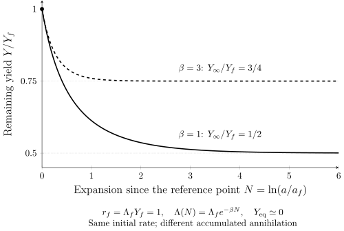
Exact post-freeze-out toy solutions with $r_f=1$, $\Lambda(N)=\Lambda_f e^{-\beta N}$, and negligible $Y_{\rm eq}$. The asymptotic yield is $Y_\infty/Y_f=1/2$ for $\beta=1$ and $3/4$ for $\beta=3$. This is chemical abundance evolution under the declared rate law, not a full thermal-relic or kinetic-decoupling prediction.

Expansion $N$	$Y/Y_f$, $\beta=1$	$Y/Y_f$, $\beta=3$
$0$	$1.0000$	$1.0000$
$1$	$0.6127$	$0.7595$
$2$	$0.5363$	$0.7505$
$\infty$	$0.5000$	$0.7500$

Common pitfalls

Equating every scattering rate with equilibration. Chemical relaxation, energy exchange, and angular isotropization are different moments of the collision operator. Use the rate that relaxes the quantity being claimed to track equilibrium.

Treating $\Gamma=H$ as an exact answer. It locates a transition only to order of magnitude. The equilibrium derivative and the integrated collision history determine the actual departure and final yield.

Assuming the standard radiation background. A modified $H(T)$, entropy release, or a separate-sector temperature changes both the crossing and the mapping from freeze-out to the later abundance.

Exercises

At temperatures well below the weak-boson masses, take $\langle\sigma v\rangle=C G_F^2T^2$ and $n_{\rm targ}=A T^3$, with dimensionless constants $A$ and $C$. During radiation domination, estimate the decoupling-temperature scaling. Then say whether an elastic reaction that conserves particle number controls chemical or kinetic decoupling.

Solution

The interaction rate is

$$\Gamma=ACG_F^2T^5,$$

while

$$H=1.66\,g_*^{1/2}\frac{T^2}{M_{\rm Pl}}.$$

Equating the two timescales gives the order-of-magnitude result

$$\boxed{ T_d =\left( \frac{1.66\,g_*^{1/2}} {ACG_F^2M_{\rm Pl}} \right)^{1/3} }.$$

The cube-root scaling is robust, but the coefficient requires the actual collision integral and a stated $g_*(T)$. Since the elastic reaction does not change particle number, it cannot by itself enforce chemical equilibrium. It controls kinetic equilibrium through momentum and energy transfer; its momentum-relaxation rate, rather than its raw collision count, must be compared with the background evolution.

References

• Gondolo, Paolo, and Graciela Gelmini. “Cosmic Abundances of Stable Particles: Improved Analysis.” Nuclear Physics B 360, no. 1 (1991): 145–179. DOI. Author-uploaded Open PDF.
• Particle Data Group. “Big-Bang Cosmology.” In Review of Particle Physics 2026. Review revised August 2025; 2026 edition dated 1 June 2026. Official PDF.
• Particle Data Group. “Dark Matter.” In Review of Particle Physics 2026. Review revised August 2025; 2026 edition dated 1 June 2026. Official PDF.
• Tong, David. Cosmology. University of Cambridge Part II Mathematical Tripos lecture notes, Michaelmas 2019. Official PDF.