Multi-Component Expansion Histories

A multicomponent universe does not jump between exact single-fluid solutions. Radiation, matter, curvature, and vacuum terms coexist, and their different powers of the scale factor determine when one overtakes another. The full history follows from one dimensionless function $E(a)=H(a)/H_0$. Equality epochs are obtained algebraically, while cosmic time requires a quadrature. This page works through both steps for a declared illustrative model and checks the result against the radiation-, matter-, and vacuum-dominated limits.

Required background. The Einstein Equation supplies the Einstein Equations and sign convention; The Friedmann Equations supplies the FLRW constraint used here; Flat-Background Hilbert Stress-Energy from Metric Variation supplies the Stress–Energy and Conservation budget for the components.

Helpful background. Relativistic Matter and Compact Objects supplies the matter and radiation closures behind the background scalings.

The component budget

Normalize the dimensionless scale factor by $a_0=1$ and define $E(a)=H(a)/H_0$. For separately conserved radiation and pressureless matter, an effective cosmological-constant density, and spatial curvature,

$$E^2(a) =\Omega_{r0}a^{-4} +\Omega_{m0}a^{-3} +\Omega_{K0}a^{-2} +\Omega_{\Lambda0}.$$

Here

$$\Omega_{K0}=-\frac{K}{H_0^2}, \qquad \Omega_{\Lambda0}=\frac{\Lambda}{3H_0^2}.$$

Evaluating at $a=1$ gives the closure check

$$E^2(1) =\Omega_{r0}+\Omega_{m0} +\Omega_{K0}+\Omega_{\Lambda0} =1.$$

Every coefficient and exponent must be declared. Massive neutrinos changing from relativistic to nonrelativistic behavior, dynamical dark energy, interactions, or additional species require replacing the corresponding simple term. The standard four-term expression is summarized in Particle Data Group 2026, §22.1.4, p. 3, eq. (22.15), and §22.2.1, p. 7, eq. (22.26) (PDF).

Equality and transition scales

Radiation–matter equality is defined by $\rho_r=\rho_m$, not by a discontinuity in either density:

$$\Omega_{r0}a_{\rm rm}^{-4} =\Omega_{m0}a_{\rm rm}^{-3}, \qquad \boxed{a_{\rm rm}=\frac{\Omega_{r0}}{\Omega_{m0}}}.$$

Matter–vacuum equality similarly occurs at

$$\boxed{ a_{m\Lambda} =\left(\frac{\Omega_{m0}}{\Omega_{\Lambda0}}\right)^{1/3} }.$$

Equality is not the onset of acceleration. For radiation, matter, and vacuum, the active gravitational sum vanishes when

$$2\Omega_{r0}a^{-4} +\Omega_{m0}a^{-3} -2\Omega_{\Lambda0}=0.$$

Neglecting radiation gives

$$\boxed{ a_{\rm acc} =\left(\frac{\Omega_{m0}} {2\Omega_{\Lambda0}}\right)^{1/3} },$$

which is smaller than $a_{m\Lambda}$. Curvature affects $H(a)$ but contributes no $\rho+3p$ term, so it does not enter this acceleration condition explicitly.

Time as a quadrature

Since $H=\dot a/a$,

$$dt=\frac{da}{aH(a)}.$$

For a big-bang branch with $t=0$ at $a=0$,

$$\boxed{ H_0t(a) =\int_0^a\frac{da'}{a'E(a')} }.$$

If the model bounces or begins at a finite scale factor, the lower endpoint and integration constant must be changed. The integral is analytic in the two big-bang limits:

$$\begin{array}{c|c|c} \text{dominant term} & H_0t(a) & \text{scale-factor behavior}\\ \hline \text{radiation} & \dfrac{a^2}{2\sqrt{\Omega_{r0}}} & a\propto t^{1/2}\\[6pt] \text{matter} & \dfrac{2a^{3/2}}{3\sqrt{\Omega_{m0}}} & a\propto t^{2/3}. \end{array}$$

Thus $Ht=1/2$ and $2/3$ in pure radiation and matter eras, respectively. A pure-vacuum model with $\Omega_{\Lambda0}\gt0$ on its expanding branch has

$$H_0(t-t_\star) =\frac{\ln(a/a_\star)}{\sqrt{\Omega_{\Lambda0}}},$$

so $a\to0$ only as $t\to-\infty$: it has no finite big-bang age, and $t_\star$ fixes an arbitrary time origin. For a flat matter–vacuum model with both densities positive, the expanding big-bang solution is

$$a(t) =\left(\frac{\Omega_{m0}}{\Omega_{\Lambda0}}\right)^{1/3} \sinh^{2/3}\left( \frac32H_0\sqrt{\Omega_{\Lambda0}}\,t \right).$$

Differentiating this expression reproduces $E^2=\Omega_{m0}a^{-3}+\Omega_{\Lambda0}$, so it is a useful analytic quadrature benchmark. Its late exponential limit also requires positive $\Lambda$. Tong develops the same dominance limits and matter–vacuum solution in Tong 2019, §§1.3.1 and 1.3.3, pp. 32–35 and 40–44 (PDF).

A declared radiation–matter–vacuum example

Choose, only for this worked calculation,

$$\Omega_{r0}=9.0\times10^{-5}, \qquad \Omega_{m0}=0.30000, \qquad \Omega_{\Lambda0}=0.69991, \qquad \Omega_{K0}=0.$$

These illustrative values sum exactly to one at the displayed precision; they are not asserted as a current parameter fit. The algebraic scales are

$$a_{\rm rm}=3.0000\times10^{-4}, \qquad a_{m\Lambda}=0.753980.$$

Solving the radiation-inclusive acceleration equation gives

$$a_{\rm acc}=0.598634,$$

whereas neglecting radiation gives $0.598434$. The small difference is a controlled consequence of radiation’s positive active gravitational mass.

To visualize the continuous transitions, define the instantaneous fractions $f_i(a)=\rho_i(a)/[\rho_r(a)+\rho_m(a)+\rho_\Lambda]$. They are obtained by dividing the corresponding terms in $E^2(a)$ by their sum. In the figure, compare point $A$ with $B$: acceleration begins when vacuum is still less abundant than matter.

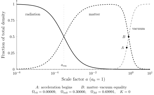
Density fractions in the illustrative flat model specified above, with a logarithmic scale-factor axis. Radiation–matter equality occurs at $a_{\rm rm}=0.0003$. Point $A$ marks acceleration at $a=0.598634$; $B$ marks matter–vacuum equality at $a=0.753980$. The fractions sum to one. These are calculated model curves, not a fit to data.

Epoch	Scale factor	Radiation fraction	Matter fraction	Vacuum fraction
Radiation–matter equality	$0.000300$	$0.500000$	$0.500000$	Less than $4\times10^{-11}$
Acceleration begins	$0.598634$	$0.000334$	$0.666222$	$0.333445$
Matter–vacuum equality	$0.753980$	$0.000199$	$0.499901$	$0.499901$
Reference present	$1$	$0.000090$	$0.300000$	$0.699910$

Rounded fractions can differ from an exact unit sum in their last digit.

For numerical quadrature, rewrite the age integrand as

$$\frac{1}{aE(a)} =\frac{a}{ \sqrt{\Omega_{r0}+\Omega_{m0}a +\Omega_{K0}a^2+\Omega_{\Lambda0}a^4} }.$$

This form has the regular endpoint value zero at $a=0$ and avoids separately evaluating large inverse powers. Composite Simpson integration on $0\leq a\leq1$ gives:

Equal panels	$H_0t_0$
4,096	0.963700427
8,192	0.963700453
16,384	0.9637004555
32,768	0.9637004557

The stabilization under panel doubling is the numerical check; the result is a dimensionless age, so conversion to time requires the separately declared $H_0^{-1}$. Early in the same calculation the radiation term gives the $t^{1/2}$ asymptote, while at large $a$ the constant term approaches exponential expansion.

Panel doubling checks convergence but not the equation being integrated. An independent test sets $(\Omega_{m0},\Omega_{\Lambda0})=(0.3,0.7)$ and uses $a=x^2$ to regularize the matter-dominated endpoint. Composite Simpson integration with 4,096 panels then gives $H_0t_0=0.964099381639468$, while the exact result is

$$H_0t(a) =\frac{2}{3\sqrt{\Omega_{\Lambda0}}} \operatorname{arsinh}\left[ \sqrt{\frac{\Omega_{\Lambda0}}{\Omega_{m0}}} a^{3/2} \right],$$

which gives $0.964099381639469$ at $a=1$. Agreement at the displayed precision checks both the quadrature and its normalization.

An executable implementation must add integration and distance-conversion tolerances, record all parameter choices, and retain convergence evidence. This page supplies the analytic equations and benchmark values that the implementation must recover.

Common pitfalls

Dominance is not exclusivity. At equality, both named components matter, and the remaining terms need not vanish. Piecewise pure-fluid solutions are asymptotic approximations, not a continuous exact history.

Equality and acceleration answer different questions. Equality compares two densities. Acceleration weights each pressure through $\rho+3p$.

A parameter list needs closure. If the displayed present-day coefficients do not sum to one, either curvature or another component is missing, or the normalization $E(1)=1$ has not been respected.

Exercises

Verify the exact flat matter–vacuum solution by differentiating it and recovering the Friedmann equation.

Solution

Let

$$C=\left(\frac{\Omega_{m0}}{\Omega_{\Lambda0}}\right)^{1/3}, \qquad x=\frac32H_0\sqrt{\Omega_{\Lambda0}}\,t, \qquad a=C\sinh^{2/3}x.$$

Then

$$H=\frac{\dot a}{a} =H_0\sqrt{\Omega_{\Lambda0}}\coth x.$$

Also

$$\Omega_{m0}a^{-3} =\Omega_{\Lambda0}\sinh^{-2}x.$$

Using $\coth^2x=1+\sinh^{-2}x$ gives

$$\frac{H^2}{H_0^2} =\Omega_{\Lambda0} +\Omega_{m0}a^{-3},$$

which is the required flat Friedmann equation. As $x$ becomes small, $\sinh x\simeq x$ and $a\propto t^{2/3}$; at large $x$, $\sinh x\propto e^x$ and the solution approaches de Sitter expansion.

Using the illustrative parameters, derive the two equality scales and explain why neither equals the acceleration scale.

Solution

Radiation–matter equality gives

$$a_{\rm rm} =\frac{9.0\times10^{-5}}{0.30000} =3.0000\times10^{-4}.$$

Matter–vacuum equality gives

$$a_{m\Lambda} =\left(\frac{0.30000}{0.69991}\right)^{1/3} =0.753980.$$

The acceleration condition instead contains pressure weights: $2\rho_r+\rho_m-2\rho_\Lambda=0$. Solving it gives $a_{\rm acc}=0.598634$. Equality compares two selected density terms, whereas acceleration tests the total active gravitational combination, so there is no reason for the scales to coincide.

References

• Particle Data Group. “Big-Bang Cosmology.” In Review of Particle Physics 2026, revised August 2025. Official PDF.
• Tong, David. Cosmology. University of Cambridge Part II Mathematical Tripos lecture notes, Michaelmas 2019. Official PDF.