Formation from Enhanced Density Perturbations

Primordial black holes can form when an unusually large, horizon-scale cosmological perturbation defeats pressure support and creates a trapped region. The decisive quantity is not a pointwise density contrast alone: it is a smoothed, slicing-specific mass excess whose collapse threshold depends on the perturbation profile and the background equation of state. That dependence is crucial because formation samples an exponentially rare tail of the primordial distribution.

Helpful background. Einstein Equations supplies the gravitational constraints; Relativistic Matter and Compact Objects supplies the perfect-fluid closure; Black-Hole Dynamics and Collapse supplies trapped surfaces and critical collapse; Relativistic Cosmology supplies the expanding background and perturbations; and Probability and Statistical Inference supplies tail probabilities and selection-aware inference.

Compaction on an expanding radiation background

Consider a spherically symmetric perturbation of a spatially flat FLRW universe filled by a perfect fluid, $p=w\rho$, with comoving radial label $r$ and areal radius $R(r,t)$. Let $M(r,t)$ be the Misner–Sharp mass and $M_b=4\pi\rho_bR^3/3$ the mass of the unperturbed background inside the same areal sphere. Restoring $G$, define the compaction function

$$\mathcal C(r,t)=\frac{2G\,[M(r,t)-M_b(r,t)]}{R(r,t)}.$$

It measures twice the excess gravitational mass in units of the areal radius. On a comoving slice and at leading order in the superhorizon gradient expansion, a curvature profile $K(r)$ gives

$$\mathcal C(r)=f(w)K(r)r^2, \qquad f(w)=\frac{3(1+w)}{5+3w}.$$

The symbol $K(r)$ is a local curvature profile, not the constant spatial curvature of the unperturbed FLRW model. To connect compaction to a more familiar density variable, define the enclosed average contrast by $\overline\delta=(M-M_b)/M_b$. The background Friedmann equation gives $\mathcal C=(HR)^2\overline\delta$. Thus compaction equals the enclosed contrast when the chosen sphere has $HR=1$; away from that time the two quantities differ. The long-wavelength amplitude labels the initial profile, while the actual collapse decision requires its nonlinear evolution.

The characteristic radius $r_m$ is the innermost relevant maximum, $\mathcal C'(r_m)=0$, and the perturbation amplitude is $\delta_m\equiv\mathcal C(r_m)$. Collapse simulations then calibrate a profile- and equation-of-state-dependent threshold $\delta_c$. On the type-I branch, where areal radius increases monotonically outward, configurations with $\delta_m\gt\delta_c$ collapse and subcritical configurations disperse. Type II instead labels a nonmonotonic areal-radius branch; it is not another name for “supercritical.” This construction, including the distinction between the curvature profile and nonlinear compaction, is developed in Escrivà, Kühnel, and Tada 2025, §§ II.C–II.E, printed pp. 12–29.

The curvature-profile width matters. A useful dimensionless measure is

$$q=-\frac{r_m^2\mathcal C''(r_m)}{4\mathcal C(r_m)}.$$

Broad peaks have small $q$ and weaker pressure gradients; sharp peaks have large $q$ and stronger gradients. In radiation domination, simulations summarized in the same review span roughly $0.4\lesssim\delta_c\lesssim2/3$ across controlled profile families. Those values are not interchangeable unless the slice, amplitude variable, profile, and horizon-entry prescription are also matched.

This also explains why the central value $\delta(0)$ is a poor universal collapse coordinate. Two profiles can share the same central density while enclosing different excess masses and presenting different pressure gradients near their edges. Compaction retains the radial information needed to locate the dynamically relevant scale, although even its peak value does not erase all profile dependence.

From a curvature spectrum to a rare collapse fraction

Use the site comoving-curvature variable $\mathcal R$. For an adiabatic regular mode, $\mathcal R\simeq\zeta$ on superhorizon scales, but the two symbols are not interchangeable at finite wavelength. Fix the spatial Fourier and power-spectrum conventions by

$$\mathcal R(\boldsymbol x) =\int\frac{d^3k}{(2\pi)^3}\, \mathcal R(\boldsymbol k)e^{i\boldsymbol k\cdot\boldsymbol x},$$ $$\langle\mathcal R(\boldsymbol k)\mathcal R(\boldsymbol k')\rangle =(2\pi)^3\delta^{(3)}(\boldsymbol k+\boldsymbol k') \frac{2\pi^2}{k^3}\mathcal P_{\mathcal R}(k).$$

For an adiabatic radiation perturbation on a comoving slice, write the linear density contrast as

$$\delta_\ell(\boldsymbol k,\eta) =\frac49\left(\frac{k}{\mathcal H}\right)^2 T\!\left(\frac{k\eta}{\sqrt3}\right) \mathcal R(\boldsymbol k), \qquad T(y)=3\frac{\sin y-y\cos y}{y^3},$$

where $\mathcal H=aH=1/\eta$ in ideal radiation domination and $T(y)\to1$ as $y\to0$. The transfer factor is essential once modes inside the smoothing integral have begun acoustic evolution. After choosing a comoving smoothing radius $R_s$ and window $W(kR_s)$, evaluate at $\mathcal H_s=R_s^{-1}$ to obtain

$$\sigma_\delta^2(R_s) =\int d\ln k\;W^2(kR_s) \frac{16}{81}(kR_s)^4 T^2\!\left(\frac{kR_s}{\sqrt3}\right) \mathcal P_{\mathcal R}(k).$$

This is the horizon-entry expression in Green and Kavanagh 2021, § II.A.4, printed pp. 4–5, Eqs. (6)–(7), translated from their source notation to the site $\mathcal R$ convention.

The random variable in this variance is linear, whereas $\delta_m$ above is the nonlinear compaction peak. For a spherical long-wavelength type-I profile, let $\delta_{\ell,m}$ denote the linearized compaction peak at the same $r_m$. Then

$$\delta_m =\delta_{\ell,m}-\frac{\delta_{\ell,m}^2}{4f(w)}, \qquad \delta_{\ell,c} =2f(w)\left[1-\sqrt{1-\frac{\delta_c}{f(w)}}\right].$$

The displayed $1-\sqrt{\cdots}$ root is the type-I branch and requires $0\le\delta_c\le f(w)$; for $\delta_c<f(w)$ the other algebraic root has $\delta_{\ell,c}>2f(w)$ and belongs to type II, with the roots meeting at the branch boundary $\delta_c=f(w)$. In radiation domination, $f=2/3$ and $\delta_m=\delta_{\ell,m}-3\delta_{\ell,m}^2/8$. A window-smoothed $\delta_\ell$ can use $\delta_{\ell,c}$ only when its window, radius, profile prescription, and horizon-entry rule match that calibration.

This nonlinear-to-linear threshold map is Escrivà, Kühnel, and Tada 2025, § II.C, printed pp. 15–17, especially Eq. (II.19), restricted here to the type-I branch and translated to the page’s amplitude notation.

For a Gaussian density $p_\ell(\delta_\ell)$, distinguish the literal one-point tail probability, the conventional Press–Schechter assignment, and the formation energy fraction:

$$P_{\rm tail}(R_s) =\int_{\delta_{\ell,c}}^{\infty} \frac{d\delta}{\sqrt{2\pi}\sigma_\delta} \exp\!\left(-\frac{\delta^2}{2\sigma_\delta^2}\right).$$ $$F_{\rm PS}(R_s)=2P_{\rm tail}(R_s), \qquad \beta_H(R_s) =2\int_{\delta_{\ell,c}}^{\delta_{\ell,\max}} d\delta\;\frac{M(\delta)}{M_H}\,p_\ell(\delta).$$

The factor two is the Press–Schechter cloud-in-cloud bookkeeping convention; it is not part of the literal Gaussian probability. Here $\beta_H$ is the mass fraction assigned per Hubble patch at the reference crossing epoch. The upper limit retains only amplitudes for which the chosen mass and collapse calibration applies. In particular, the type-I map above requires $\delta_{\ell,\max}\le2f(w)$; integrating that map to infinity would include the other branch and eventually give an unphysical negative compaction. Type-II configurations require a separate treatment, not an extrapolation.

If one assigns the constant mass $M=\alpha M_H$ on this bounded branch, then $\beta_H=2\alpha P_{\rm branch}$, where $P_{\rm branch}=\int_{\delta_{\ell,c}}^{\delta_{\ell,\max}}p_\ell\,d\delta$. The familiar $\beta_H\simeq\alpha F_{\rm PS}$ additionally neglects the Gaussian probability beyond the upper limit. Omitting $M/M_H$ silently turns an energy fraction into an assigned collapse fraction. Transport from the crossing reference to a later population is derived in Horizon Mass, Critical Collapse, and Mass Functions.

For $\nu_c=\delta_{\ell,c}/\sigma_\delta\gg1$, the leading Gaussian tail is $P_{\rm tail}\propto\nu_c^{-1}e^{-\nu_c^2/2}$. Thus threshold uncertainty is amplified exponentially. As a controlled toy comparison, express both thresholds in the same linear variable. At fixed $\sigma_\delta=0.08$, changing only $\delta_{\ell,c}$ from $0.45$ to $0.55$ changes the leading exponential by

$$\frac{P_{\rm tail}(0.55)}{P_{\rm tail}(0.45)} \approx \exp\!\left[-\frac{0.55^2-0.45^2}{2(0.08)^2}\right] =4.05\times10^{-4}.$$

The probability falls by more than three orders of magnitude. The figure evaluates the full Gaussian integral at the same fixed variance; inspect the vertical separation on the logarithmic scale. The exact ratio is $3.34\times10^{-4}$, compared with $4.05\times10^{-4}$ when only the leading exponential is kept.

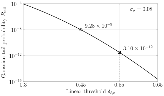
For the same Gaussian linear variable with $\sigma_\delta=0.08$, the literal tail falls by more than three orders of magnitude between thresholds $0.45$ and $0.55$. The vertical scale is logarithmic. These are quantitative toy probabilities, without a Press–Schechter factor or PBH mass weighting; the thresholds do not represent a fitted physical uncertainty interval.

Linear threshold $\delta_{\ell,c}$	Literal Gaussian tail $P_{\rm tail}$
$0.45$	$9.2754\times10^{-9}$
$0.55$	$3.0995\times10^{-12}$

Neither the plotted probability nor its ratio includes the amplitude-dependent mass weight required to predict $\beta_H$.

A second check isolates smoothing. For a monochromatic $\mathcal P_{\mathcal R}=A\,\delta_{\rm D}[\ln(k/k_*)]$ with $k_*R_s=1$, compare a real-space top-hat, $W_{\rm TH}(x)=3(\sin x-x\cos x)/x^3$, with $W_{\rm G}(x)=e^{-x^2/2}$. The common transfer factor cancels in their ratio:

$$\frac{\sigma_{\rm TH}}{\sigma_{\rm G}} =\frac{W_{\rm TH}(1)}{W_{\rm G}(1)} =\frac{0.9035}{0.6065}=1.490.$$

If the Gaussian-window significance is $\nu_{\rm G}=6$, then $\nu_{\rm TH}=4.028$ and the leading-tail estimate gives $P_{\rm tail,TH}/P_{\rm tail,G}\simeq2.93\times10^4$. This is not a physical prediction: it demonstrates why a threshold must be calibrated with its own window and profile. Green and Kavanagh 2021, §§ II.A.1–II.A.4, printed pp. 3–5 compare these conventions.

Results and limitations through 2026-08-19

The status as of 2026-08-19 is conditional rather than a universal verdict. Relativistic collapse is well established for specified initial data, but the mapping from a primordial stochastic field to those data remains formulation-dependent.

Formulation or evidence	Result	Scope and limitation
Long-wavelength compaction plus relativistic fluid simulations	A profile-dependent threshold separates collapse from dispersal, and critical scaling appears near threshold	Requires a declared comoving slicing, equation of state, profile family, numerical domain, and horizon-entry convention
Gaussian Press–Schechter-like tail	Gives a transparent exponential estimate for $\beta$	Treats one smoothed variable as Gaussian, uses a cloud-in-cloud prescription, and does not count peaks geometrically
Peak theory for $\zeta$ or $\nabla^2\zeta$	Connects spectral moments to peak profiles and number density	Results depend on which peaks are counted, the window, environmental modes, and the collapse calibration
Non-Gaussian tail statistics	Even modest changes to the far tail can alter abundance by many orders of magnitude	A low-order cumulant or local expansion need not control the rare tail at amplitudes of order unity

The credible competing positions are therefore not “collapse occurs” versus “collapse does not occur.” They concern how peak theory, Press–Schechter-like estimates, compaction-threshold simulations, critical collapse, and non-Gaussian tail models should be joined for a specified power spectrum. The strongest unresolved issue is a controlled end-to-end map from inflationary statistics through smoothing and nonlinear initial data to a calibrated abundance over broad spectra and nonspherical initial data.

The interpretation could change after new relativistic collapse simulations jointly calibrate profile and nonsphericity over a broad spectral family, or after a nonperturbative tail-statistics calculation changes the abundance mapping while holding the same initial curvature ensemble fixed.

A diagnostic for threshold claims

Suppose two studies use the same quoted $\mathcal P_{\mathcal R}(k)$ but obtain different PBH abundances. What must be checked before interpreting the difference as a physical disagreement?

Solution

First compare their Fourier and power-spectrum normalizations. Then match the smoothing window and radius, the slicing and density variable, the curvature-to-density transfer at horizon entry, and the definition of horizon crossing. Next compare the perturbation profile or peak prescription, equation of state, the map between $\delta_c$ and $\delta_{\ell,c}$, and the numerical collapse calibration. Finally compare the assumed probability tail and the mass weight $M/M_H$, including non-Gaussianity and critical collapse. Because a rare tail is exponentially sensitive to $\delta_{\ell,c}/\sigma_\delta$, a mismatch in any one of these choices can generate orders-of-magnitude disagreement without representing different physics.

Scope boundary

This page establishes the formation probability from enhanced density perturbations. It does not derive the general theory of critical phenomena, replace a nonlinear collapse simulation, or turn a formation fraction into a present dark-matter fraction. Mass Scaling and Critical Exponents develops the general critical-collapse law; the cosmological mass mapping belongs to the next page. Evaporation, population evolution, and observational constraints require additional physics developed later in this chapter.

References

• Escrivà, Albert, Florian Kühnel, and Yuichiro Tada. 2025. “Primordial Black Holes.” arXiv:2211.05767v5. Open PDF.
• Green, Anne M., and Bradley J. Kavanagh. 2021. “Primordial Black Holes as a Dark Matter Candidate.” Journal of Physics G 48: 043001. DOI.