Quantizing Primordial Perturbations

Inflation turns each linear perturbation mode into a harmonic oscillator with a time-dependent frequency. Quantization therefore requires three ingredients that must not be conflated: the correctly normalized canonical variable, its commutator, and a choice of quantum state. In the canonical single-field attractor considered here, an adiabatic short-wavelength state evolves into a highly squeezed state whose long-wavelength curvature amplitude is nearly constant. More general backgrounds or initial states need not share that last step.

Required background. The Einstein Equation supplies Einstein Equations for eliminating lapse and shift constraints. Classical Field Modes and Canonical Variables supplies Flat-Spacetime Quantum Field Theory for canonical commutators, positive-frequency modes, and Fourier normalization.

Helpful background. Relativistic Matter and Compact Objects supplies stress–energy variables, while Relativistic Cosmology supplies the inflationary FLRW background. Bardeen Potentials and Curvature Perturbations fixes the sign of $\mathcal R$ used here.

The canonical scalar degree of freedom

Work on a monotonic segment of a spatially flat background with one canonical scalar field, $\dot\phi\ne0$, $H\ne0$, and no independent entropy mode. Dots denote cosmic-time derivatives; primes denote conformal-time derivatives, with $d\eta=dt/a$ and $\mathcal H=aH$. Let $M=(8\pi G)^{-1/2}$ and define

$$z\equiv\frac{a\dot\phi}{H} =\frac{a\phi'}{\mathcal H}, \qquad z^2=2a^2M^2\epsilon_H.$$

The sign of $z$ follows the sign of $\dot\phi$; only $z^2$ enters the curvature action. This site defines

$$\mathcal R=-\psi+\mathcal H\frac{\delta q}{\rho+p}.$$

For a canonical scalar, $\delta q=-(\rho+p)\delta\phi/\phi'$, so $\mathcal R=-\psi-\mathcal H\delta\phi/\phi'$. This is the negative of the curvature variable denoted $\mathcal R$ in Baumann’s lectures. To preserve the standard canonical mode while retaining the site’s curvature sign, define

$$\boxed{v\equiv-z\mathcal R}.$$

Equivalently, $v=a[\delta\phi+(\phi'/\mathcal H)\psi]$ is the scale-factor rescaling of the field perturbation on spatially flat slices. Eliminating the lapse and shift does not discard another propagating scalar wave: those variables impose constraints, leaving this single physical scalar oscillator.

After the nondynamical scalar constraints have been removed, the quadratic action is

$$S^{(2)}_{\rm s} =\frac12\int d\eta\,d^3x\, z^2\left[(\mathcal R')^2-(\nabla\mathcal R)^2\right]$$

or, after integrating one boundary term,

$$S^{(2)}_{\rm s} =\frac12\int d\eta\,d^3x \left[(v')^2-(\nabla v)^2+\frac{z''}{z}v^2\right].$$

With $v(\eta,\mathbf x)=\int d^3k\,v_{\mathbf k}(\eta) e^{i\mathbf k\cdot\mathbf x}/(2\pi)^3$, each mode satisfies the Mukhanov–Sasaki equation

$$v_k''+\left(k^2-\frac{z''}{z}\right)v_k=0.$$

The action, mode equation, and source convention are derived in Baumann 2012, §§12.2.1–12.2.2, printed pp. 56–57, eqs. (179)–(189) (Open PDF). The overall replacement $\mathcal R_{\rm here}=-\mathcal R_{\rm source}$ leaves the quadratic action and all power spectra unchanged.

Commutator and Wronskian

Set $\hbar=1$ and promote $v$ to a Hermitian operator,

$$\widehat v(\eta,\mathbf x) =\int\frac{d^3k}{(2\pi)^3} \left[ v_k(\eta)\widehat a_{\mathbf k}e^{i\mathbf k\cdot\mathbf x} +v_k^*(\eta)\widehat a_{\mathbf k}^{\dagger} e^{-i\mathbf k\cdot\mathbf x} \right].$$

The conjugate momentum is $\widehat\pi_v=\widehat v'$. Requiring

$$[\widehat v(\eta,\mathbf x),\widehat\pi_v(\eta,\mathbf y)] =i\delta^{(3)}(\mathbf x-\mathbf y),$$

together with $[\widehat a_{\mathbf k},\widehat a_{\mathbf q}^{\dagger}] =(2\pi)^3\delta^{(3)}(\mathbf k-\mathbf q)$, fixes the mode Wronskian:

$$\boxed{ v_kv_k^{*\prime}-v_k^*v_k'=i }.$$

The Wronskian is conserved by the real second-order mode equation. It fixes the normalization, but not the state: a Bogoliubov-rotated pair of solutions can obey the same Wronskian.

The adiabatic short-wavelength state

When

$$k^2\gg\left\lvert\frac{z''}{z}\right\rvert$$

and the effective frequency varies adiabatically, the mode behaves locally as a Minkowski oscillator. The Bunch–Davies prescription selects

$$v_k(\eta)\longrightarrow\frac{e^{-ik\eta}}{\sqrt{2k}}, \qquad \widehat a_{\mathbf k}\lvert0\rangle=0.$$

This is a physical state assumption. It is well motivated if the mode can be continued far enough into an adiabatic sub-Hubble regime. A finite onset of inflation, a nonadiabatic background, an excited initial state, or physics near the effective-theory cutoff can prevent that argument from selecting a unique state. Baumann makes the vacuum nonuniqueness and the Bunch–Davies condition explicit in Baumann 2012, §§11.2–11.3 and §12.2.3, printed pp. 52–57, eqs. (157)–(176) and (186)–(192) (Open PDF).

For slowly varying $\epsilon_H$, one has $z''/z\simeq2/\eta^2$ at leading quasi-de Sitter order. The normalized solution is then

$$v_k(\eta)=\frac{e^{-ik\eta}}{\sqrt{2k}} \left(1-\frac{i}{k\eta}\right).$$

It is important not to call this an exact scalar result in exact de Sitter space. When $\epsilon_H=0$ exactly, the single-field clock stops, $z=0$, and comoving curvature is ill-defined. The formula is the leading quasi-de Sitter limit with nonzero, slowly varying $\epsilon_H$.

Freeze-out and its exception

For $\lvert k\eta\rvert\ll1$,

$$\lvert v_k\rvert \simeq\frac{1}{\sqrt{2k^3}\lvert\eta\rvert}.$$

Using $a\simeq-1/(H\eta)$ and $z^2=2a^2M^2\epsilon_H$ gives

$$\lvert\mathcal R_k\rvert =\frac{\lvert v_k\rvert}{\lvert z\rvert} \simeq\frac{H}{2M\sqrt{\epsilon_H}\,k^{3/2}}.$$

More generally, the curvature equation is

$$(z^2\mathcal R_k')'+k^2z^2\mathcal R_k=0.$$

At leading long-wavelength order,

$$\mathcal R_k=C_k+D_k\int^\eta\frac{d\widetilde\eta}{z^2}.$$

The second solution decays in the usual slow-roll attractor, leaving a frozen $C_k$. It can grow in a nonattractor phase—for example, when $\epsilon_H$ falls fast enough that $z$ decreases. Thus “super-Hubble curvature freezes” is a conditional dynamical result, not a definition of a long-wavelength mode.

For example, on an approximately flat potential with nearly constant $H$, the homogeneous equation gives $\dot\phi\propto a^{-3}$, hence $\epsilon_H\propto a^{-6}$ and $z\propto a^{-2}$. The second solution then scales as $\int d\eta/z^2\propto\int a^3dt\propto a^3$. A mode can therefore grow rapidly outside the Hubble radius during this ultra-slow-roll interval. The eventual amplitude must be obtained by evolving through its entrance and exit, rather than by reading the usual slow-roll formula at one crossing time.

How gradual is freeze-out?

The approximate mode solution above also gives the approach to the constant amplitude. With $x=-k\eta\gt0$ and $|\mathcal R_k|_{\rm late}=H/(2M\sqrt{\epsilon_H}\,k^{3/2})$,

$$\frac{|\mathcal R_k|}{|\mathcal R_k|_{\rm late}} =\sqrt{1+x^2}.$$

This equality belongs to the leading slow-roll mode approximation: $H$ and nonzero $\epsilon_H$ are treated as constant to that order. It does not assert an exactly de Sitter scalar background with a rolling clock field. The horizontal coordinate $\mathcal N=-\ln x\simeq\ln(a/a_{\rm cross})$ measures approximate e-folds after $k=aH$. Inspect the smooth approach to unity in the figure; there is no abrupt change at the marked crossing.

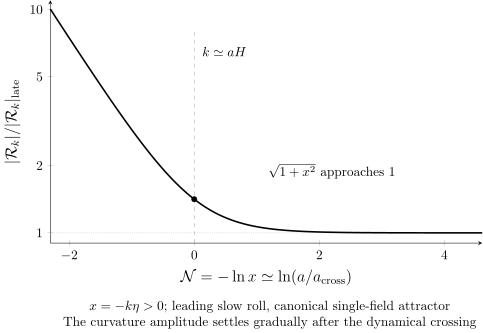
Normalized curvature amplitude $\sqrt{1+x^2}$ for the leading slow-roll, canonical single-field attractor solution in the adiabatic state, with $x=-k\eta$ and nonzero $\epsilon_H$. The amplitude axis is logarithmic. At $x=1$ the amplitude is $\sqrt2$ times its late limit; subsequent evolution approaches unity. This dynamical crossing is neither instantaneous freeze-out nor the crossing of a global causal horizon.

$x=-k\eta$	Approximate e-fold coordinate $\mathcal N$	Amplitude divided by its late limit
$10$	$-2.303$	$10.049876$
$1$	$0$	$1.414214$
$0.1$	$2.303$	$1.004988$
$0.01$	$4.605$	$1.000050$

The canonical mode $v_k$ and curvature $\mathcal R_k=-v_k/z$ have different amplitudes: outside the Hubble scale, growth of $v_k$ is compensated by the background factor $z$ in this attractor. The nonattractor example above explains why the same cancellation cannot be assumed for every inflationary history.

Tensor oscillators

Write the transverse-traceless metric perturbation as

$$h_{ij}=\sum_{\lambda=+,\times} \int\frac{d^3k}{(2\pi)^3} e_{ij}^{\lambda}(\widehat{\mathbf k}) h_{\lambda,\mathbf k}e^{i\mathbf k\cdot\mathbf x},$$

with $e_{ij}^{\lambda}e^{\lambda'ij}=2\delta_{\lambda\lambda'}$. The quadratic Einstein–Hilbert action is

$$S^{(2)}_{\rm t} =\frac{M^2}{8}\int d\eta\,d^3x\,a^2 \left[(h_{ij}')^2-(\nabla h_{ij})^2\right].$$

For each polarization, the canonical variable

$$u_\lambda\equiv\frac{aM}{\sqrt2}h_\lambda$$

obeys

$$u_{\lambda,k}''+ \left(k^2-\frac{a''}{a}\right)u_{\lambda,k}=0, \qquad u_{\lambda,k}u_{\lambda,k}^{*\prime} -u_{\lambda,k}^*u_{\lambda,k}'=i.$$

The two independent polarizations therefore have the same leading Bunch–Davies mode as a massless canonical oscillator in quasi-de Sitter space. The factor $\sqrt2$ follows directly by inserting the norm-two polarization contraction into the action before normalizing each real plus/cross field. Caprini and Figueroa 2018, §5.1.2, printed p. 64 and pp. 67–68, eqs. (167)–(171) and (185)–(191) (Open PDF) use the same direct plus/cross decomposition, norm-two basis, tensor action, canonical variable, and contracted inflationary spectrum after identifying their reduced Planck mass with $M$. Baumann 2012, §12.3, printed pp. 60–61, eqs. (208)–(216) (Open PDF) supplies an independent derivation, but only its final contracted spectrum is used as a cross-check: its displayed canonical component and one-polarization spectrum are normalized differently. The canonical factor here is fixed by the direct action substitution together with this page’s explicit full-space covariance and Wronskian; a component-mode rescaling cannot be imported independently of those definitions.

What “classical-looking” means

Outside the Hubble radius, the growing and decaying phase-space directions become extremely unequal: the state is highly squeezed and the surviving field amplitude has nearly fixed phase. Its equal-time Gaussian correlations can then be represented by a classical stochastic field with the same two-point function. Unitary squeezing alone does not select one realized field configuration or prove environmental decoherence. Interactions, unobserved degrees of freedom, and a coarse-graining prescription are needed for that stronger claim.

The curved-spacetime construction, adiabatic-state criteria, and particle interpretation are developed more deeply in Inflationary Fluctuations as Curved-Spacetime Fields. The next page fixes the scalar and tensor two-point normalizations and extracts their observable spectra.

Exercises

Verify both the Wronskian and the long-wavelength curvature amplitude for the quasi-de Sitter Bunch–Davies mode.

Solution

Substituting

$$v_k=\frac{1-i/(k\eta)}{\sqrt{2k}}e^{-ik\eta}$$

and its derivative gives $v_kv_k^{*\prime}-v_k^*v_k'=i$ at every $\eta$. At $\lvert k\eta\rvert\ll1$,

$$\lvert v_k\rvert^2\longrightarrow\frac{1}{2k^3\eta^2}.$$

Since $\lvert\mathcal R_k\rvert^2=\lvert v_k\rvert^2/z^2$ and

$$z^2=2a^2M^2\epsilon_H \simeq\frac{2M^2\epsilon_H}{H^2\eta^2},$$

one finds

$$\lvert\mathcal R_k\rvert^2 \simeq\frac{H^2}{4M^2\epsilon_Hk^3}.$$

The sign in $v=-z\mathcal R$ drops out of this two-point normalization but is still essential when comparing signed transfer relations across conventions.

References

• Baumann, D., “TASI Lectures on Inflation,” arXiv:0907.5424v2 (2012), Open PDF.
• Caprini, C., and D. G. Figueroa, “Cosmological Backgrounds of Gravitational Waves,” Classical and Quantum Gravity 35, 163001 (2018), DOI, Open PDF.
• Ellis, J., V. Vennin, and D. Wands, “Inflation,” in F. Takahashi et al. (Particle Data Group), Review of Particle Physics, International Journal of Modern Physics A 41, 2630011 (2026), revised August 2025, Official PDF.