Coordinate Domains and Horizon Structure

A C-metric line element becomes a Lorentzian spacetime only after one chooses a connected domain on which its structure functions have the required signs. In the standard vacuum sector $0<2mA<1$, the root ordering selects a static rectangle bounded by two axes, a black-hole horizon, and an acceleration horizon. Other rectangles describe extensions or different components; they cannot be combined by retaining the same labels without checking signature and boundary identifications.

Required background. Killing Fields and Isometry Groups supplies Killing horizons and axial fixed sets.

Helpful background. The Einstein Equation supplies the vacuum equations; The Riemann Curvature Tensor distinguishes singular endpoints; Exact Solutions of Einstein’s Equations places the family; Global Structure develops extensions and conformal boundaries; and Frames, Coframes, and Anholonomy supplies regular frames.

Root ordering and Lorentzian signature

Use

$$G(\xi)=(1-\xi^2)(1+2mA\xi), \qquad F(y)=-G(y),$$

and set $\alpha=2mA$. For $0<\alpha<1$, the three ordered roots are

$$\xi_1=-\frac1\alpha<-1=\xi_2<1=\xi_3.$$

For $G(x)>0$ and $F(y)\ne0$, the factorized metric has one timelike direction because the $(\tau,y)$ block has determinant $-1$ before the positive conformal rescaling. The condition $F(y)>0$ specifically makes $\partial_\tau$ timelike; when $F(y)<0$, $y$ is timelike instead. The standard static rectangle is

$$-1<x<1, \qquad -\frac1\alpha<y<-1.$$

Indeed $G(x)>0$ on the angular interval. On the $y$ interval, $1-y^2<0$ while $1+\alpha y>0$, so $G(y)<0$ and $F(y)>0$. The Killing field $\partial_\tau$ is timelike there.

Under $x=\cos\theta$ and $y=-1/(Ar)$, this rectangle becomes

$$0<\theta<\pi, \qquad 2m<r<\frac1A.$$

The restriction $0<\alpha<1$ is therefore exactly $2m<A^{-1}$: the black-hole and acceleration horizons are distinct and enclose a nonempty static radial interval.

The figure turns the inequalities into a domain map. First follow the signs across the ordered roots; then use the highlighted $x$ and $y$ intervals as the horizontal and vertical directions of the static cell. The dotted line marks where the compactifying factor $A(x-y)$ vanishes and the physical-metric prefactor diverges, not a fifth side of the open rectangle.

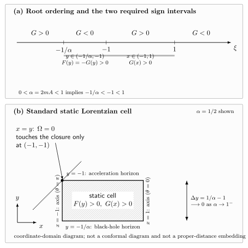
For $0<\alpha=2mA<1$, $G>0$ on $(-1,1)$ while $F=-G>0$ on $(-1/\alpha,-1)$. These intervals form the standard static Lorentzian cell, bounded by the axes $x=\pm1$, black-hole horizon $y=-1/\alpha$, and acceleration horizon $y=-1$. Conformal infinity $x=y$ meets its closure only at $(-1,-1)$, and the coordinate width $1/\alpha-1$ vanishes as $\alpha\to1^-$. Panel (b) uses $\alpha=1/2$; it is a coordinate-domain diagram, not a conformal or proper-distance diagram.

Axes, horizons, and conformal infinity

The boundaries have different geometric meanings:

• $x=1$ and $x=-1$ are fixed-point sets of the axial Killing field. Local regularity there depends on the period of $\phi$.
• $y=-1/\alpha$ maps to $r=2m$, where the static Killing field becomes null. It is the black-hole Killing horizon in this domain.
• $y=-1$ maps to $r=A^{-1}$ and is the acceleration Killing horizon.
• $x=y$ makes the conformal prefactor singular and corresponds to $\Omega=1+Ar\cos\theta=0$ in spherical variables.

Within the open static rectangle, $y<-1<x$, so $x=y$ is absent. Its closure meets conformal infinity at the corner $x=y=-1$, or $r=A^{-1}$ and $\theta=\pi$. Extensions through the acceleration horizon expose a larger portion of the conformal boundary. This corner behavior is why a rectangular coordinate diagram should not be read as a conformal diagram without further analysis.

A simple zero of $F$ is a coordinate degeneracy of the static chart. Introduce an ingoing coordinate

$$v=\tau+\int\frac{dy}{F(y)}.$$

Then the $(\tau,y)$ sector becomes $-Fdv^2+2\,dv\,dy$, up to the common conformal factor, and is regular at a simple root provided the conformal factor and transverse metric remain finite. Curvature invariants decide whether any particular endpoint is also singular.

Domain changes at degeneracy

At $\alpha=1$, the roots $-1/\alpha$ and $-1$ coincide. Equivalently $2m=1/A$, so the static interval collapses. A meaningful near-degenerate geometry may still be obtained by scaling the radial and time coordinates around the double root, but it is not found by merely setting $\alpha=1$ in a chart whose open domain has disappeared.

When $\alpha>1$, the root $-1/\alpha$ moves between $-1$ and $0$ and enters the usual angular range. The interval $-1<x<1$ no longer has $G>0$ throughout, so the familiar two-axis spherical interpretation fails. One must reselect connected sign intervals and re-evaluate their topology and conicities. This is a change of admissible domain, not just a numerical continuation of the standard accelerating-black-hole exterior.

Charge, rotation, and $\Lambda$ produce quartic structure functions or alter their roots. The same method survives: order the real roots, build a sign chart, exclude zeros of the conformal factor from the interior, and identify each boundary through Killing norms, fixed sets, and invariants. Discriminants mark parameter values where the domain decomposition changes.

Horizon checks and scope

In spherical variables the radial function is

$$Q(r)=(1-A^2r^2)(1-2m/r).$$

Both simple roots can be crossed by horizon-penetrating coordinates. A surface-gravity expression proportional to $\lvert Q'(r_h)\rvert/2$ depends on the normalization chosen for $\partial_t$; the C-metric has no single asymptotically flat static infinity that automatically fixes it. This chapter identifies the exact horizon hypersurfaces and domains, while global event horizons and thermodynamic normalizations require additional boundary information.

The curvature singularity associated with the black hole lies beyond the $r=2m$ boundary of the static rectangle. The acceleration horizon is not a curvature singularity in the vacuum family. Checking the Weyl scalar or Kretschmann invariant distinguishes these statements from coordinate inference; a systematic domain analysis is given in Griffiths, Krtouš, and Podolský 2006, §§ 2–4.

Exercises

Construct the sign chart of $G(\xi)$ for $0<\alpha<1$ and verify the signs used in the standard rectangle.

Solution

The simple roots are $-1/\alpha<-1<1$, and the leading cubic coefficient is $-\alpha<0$. Testing one point in each interval gives

$$\begin{array}{c|cccc} \xi & (-\infty,-1/\alpha) & (-1/\alpha,-1) & (-1,1) & (1,\infty)\\ \hline G(\xi) & + & - & + & - \end{array}$$

Thus $G(x)>0$ for $-1<x<1$. Choosing $y$ in $(-1/\alpha,-1)$ gives $G(y)<0$, hence $F(y)=-G(y)>0$. The resulting metric has one negative coefficient, the $d\tau^2$ term, and three positive spatial coefficients.

References

• Jerry B. Griffiths, Pavel Krtouš, and Jiří Podolský, “Interpreting the C-Metric,” Classical and Quantum Gravity 23, 6745–6766 (2006). DOI.