Constructing Penrose Diagrams

A Penrose diagram is a finite picture of a spacetime’s radial causal structure. Constructing one is not the act of squeezing a familiar coordinate plot: it is a sequence of coordinate, domain, and conformal steps whose result must be checked against the original metric. The reliable output records which radial null curves meet, which boundaries they reach, and which regions are actually part of the spacetime.

Required background. Lorentzian Metrics and Causal Cones supplies null directions and conformal invariance of cones. Helpful background. Geodesics and Jacobi Fields supplies affine and maximal extensions; Causality and Global Structure supplies the global questions a diagram answers; Exact Solutions of Einstein’s Equations supplies coordinate extensions and canonical test cases.

Radial null coordinates

For a spherically symmetric metric, suppress the symmetry spheres only after writing

$$d\widetilde s^2=\widetilde h_{AB}(x)\,dx^A dx^B+r^2(x)d\omega_2^2.$$

The diagram represents the two-dimensional orbit-space metric $\widetilde h$, while each ordinary interior point usually stands for a two-sphere. The first task is to find coordinates adapted to its two radial null families. Locally every two-dimensional Lorentzian metric is conformally flat, so one seeks $u,v$ with

$$\widetilde h=-F(u,v)\,du\,dv, \qquad F\gt0$$

on the domain under study. Radial null curves then have $u=\text{constant}$ or $v=\text{constant}$. Their slopes can conventionally be drawn at $45^\circ$, because multiplying the metric by a positive function leaves those curves null.

Coordinates that diverge at a horizon must be extended before compactification. For Schwarzschild, compactifying Schwarzschild $t$ and $r$ directly preserves the chart’s false boundary at $r=2GM$. One first uses Eddington–Finkelstein or Kruskal-type null coordinates to determine which horizon is regular and which regions are included. The maximal analytic extension, a collapse spacetime, and the exterior chart therefore yield different diagrams even though their exterior metric components overlap.

Compactify without changing causal order

Once the null ranges are known, choose smooth monotone bounded functions

$$U=f(u), \qquad V=g(v).$$

Monotonicity preserves future order along each null family. After choosing an arbitrary length $L\gt0$, the common Minkowski choice $U=\arctan(u/L)$, $V=\arctan(v/L)$ maps the real line to $(-\pi/2,\pi/2)$. With

$$T=U+V, \qquad R=V-U,$$

radial null curves remain at $45^\circ$. A conformal factor cancels the divergent coordinate prefactor. For Minkowski space,

$$\Omega=\frac{2}{L}\cos U\cos V =\frac{\cos T+\cos R}{L}$$

gives

$$ds^2=\Omega^2d\widetilde s^2 =-dT^2+dR^2+\sin^2R\,d\omega_2^2.$$

The scale $L$ is needed to make the arctangent arguments dimensionless; changing it changes no causal or boundary relation. The physical domain is not the full Einstein cylinder. From $r\geq0$ and finite $u,v$ one obtains $R\geq0$ and $-\pi\lt T\pm R\lt\pi$. Those inequalities are part of the answer: they determine the radial triangle, its axis, and its ideal boundary. Frauendiener’s explicit construction supplies a checked model Frauendiener 2004, §2.2, Eqs. (2)–(7).

Those inequalities produce the triangular radial quotient shown below, not the full diamond of signed $1+1$ Cartesian space. Inspect the regular $r=0$ center, the open null-infinity edges, and the three different ideal endpoints. The representative curves check that null, inertial-timelike, and constant-time spacelike directions terminate where the coordinate calculation says they should.

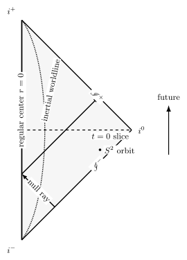
The radial compactification of four-dimensional Minkowski spacetime is a triangle: the vertical edge is the regular center, the open diagonal edges are null infinity, and the vertices are timelike or spatial ideal endpoints. Future points upward; the diagram is schematic and not to scale.

Other monotone compactifications produce diagrams with different shapes but the same causal incidence. Angles, coordinate lengths, and apparent areas have no invariant meaning. A useful diagram is therefore judged by its labels and causal relations, not by resemblance to a canonical silhouette.

Classify every boundary segment

Every line in the completed coordinate rectangle needs a geometric explanation. For a conformal boundary $\Omega=0$, compute the unphysical normal $n_a=\nabla_a\Omega$: its squared norm classifies the boundary as spacelike, null, or timelike. For a finite-coordinate metric surface, evaluate curvature, extensions, and the areal radius before calling it a singularity, axis, or horizon.

The following checks prevent the most common mislabels:

1. Center: in spherical symmetry, $r=0$ is regular only if the spheres shrink with the required smoothness and local-flatness behavior; otherwise it may be singular. A rotation axis and a spherical center have different orbit dimensions, even when both are drawn as an edge.
2. Infinity: on a regular open boundary segment verify $\Omega=0$, $d\Omega\neq0$, the unphysical metric’s regularity, and which physical curves approach it. Ideal vertices such as Minkowski $i^0$ and $i^\pm$, where $d\Omega=0$, require a separate endpoint analysis.
3. Horizon: decide whether it is a coordinate horizon, Killing horizon, Cauchy horizon, or event horizon. An event horizon additionally needs a specified $\mathscr I^+$ and the entire causal past $J^-(\mathscr I^+)$.
4. Singularity: demonstrate inextendibility or the relevant curvature/curve behavior. A jagged line is notation, not evidence.
5. Identification: if edges are identified, mark the identification; a quotient can change topology and create closed causal curves without changing the local metric.

The result should also show time orientation and the physical region. A diagram with correctly sloped null rays but an unmarked excluded wedge can assert the wrong causal accessibility.

A reproducible construction workflow

For a new spacetime, use this sequence:

• identify the manifold, coordinate ranges, symmetry orbits, and candidate extensions;
• solve the radial null equation and introduce double-null coordinates on each regular patch;
• extend across removable coordinate singularities before declaring a boundary;
• choose monotone compactifying maps and record their images;
• rescale by a positive conformal factor and test regularity;
• impose every original domain inequality in the new coordinates;
• classify axes, infinities, horizons, singular boundaries, and identifications independently;
• trace representative timelike and null curves and verify their endpoints;
• compare overlapping patches and state whether the result is maximal, exterior-only, or tied to chosen initial data.

This procedure preserves radial causal order, not the angular geometry or metric scale. Sánchez’s comparison of embeddings, causal boundaries, slicings, and counterexamples is a useful safeguard against treating a conformal picture as a unique completion Sánchez 2022, §§4–6, pp. 22–46.

A Schwarzschild domain check

Schwarzschild geometry illustrates why extension and domain analysis come before compactification. The usual static coordinates cover only one exterior region. Their time coordinate diverges when a radial null curve approaches the surface of areal radius $2GM$, even though freely falling curvature components remain finite there. If one compactifies that chart as it stands, the coordinate edge is easily mistaken for a terminal boundary.

An ingoing Eddington–Finkelstein chart crosses the future horizon and includes the black-hole interior, but it is not adapted to crossing the past horizon. An outgoing chart makes the opposite choice. Kruskal-type null coordinates cover both and reveal two exterior regions, a black-hole region, and a white-hole region in the maximally extended vacuum solution. The familiar four-region diagram is therefore a statement about that maximal extension, not about every spacetime with a Schwarzschild exterior.

A black hole formed by collapse has a different physical manifold. Before the star collapses, the regular center replaces the white-hole singularity and the second exterior. Its event horizon begins at the regular center and later joins the stationary null surface. The exterior metric at late times can be Schwarzschild while the global diagram is not the eternal one. This is a decisive counterexample to constructing a diagram from a local line element alone.

The check has three parts. First, curvature invariants separate the regular horizon from the genuine central curvature singularity. Second, radial null coordinates establish which surfaces are crossable and in which direction. Third, matching to the matter region and the selected initial data determines the spacetime domain. Only then should one compactify, label future null infinity, and define the event horizon from its causal past.

The same lesson applies beyond spherical symmetry. A two-dimensional drawing may be a quotient, a selected totally geodesic plane, or merely a schematic summary. The page or caption must say which. If the reduction does not faithfully encode every causal curve, the picture can illustrate a result proved elsewhere but cannot establish it.

Exercise

Compactify $1+1$ Minkowski spacetime with $U=\arctan[(t-x)/L]$ and $V=\arctan[(t+x)/L]$ for $L\gt0$. Locate the worldline $x=0$, the outgoing null ray $t-x=u_0$, and the constant-time line $t=0$.

Solution

For $x=0$, $u=v=t$, hence $U=V$ and $R=V-U=0$: the observer lies on the central timelike line and runs from $i^-$ to $i^+$. Here $x$ is a signed Cartesian coordinate, so this line is an interior line of the full diamond, not a boundary representing a spherical center. For $u=u_0$, $U=\arctan(u_0/L)$ is constant while $V$ increases, giving a $45^\circ$ outgoing line that ends at $V=\pi/2$, on the right-hand component of $\mathscr I^+$. For $t=0$, $v=x=-u$, so $V=-U$ and $T=U+V=0$; as $x\to+\infty$, $(U,V)\to(-\pi/2,\pi/2)$, the right spatial endpoint. The other end $x\to-\infty$ gives the left spatial endpoint. The radial $3+1$ quotient retains only the $r\geq0$ triangle and suppresses the spatial sphere of directions. These results follow from the coordinate map and domain, not from drawing convention alone.

Causal Boundary Constructions next asks how to attach ideal endpoints when a smooth conformal rescaling is unavailable.

References

• Frauendiener, Jörg, “Conformal Infinity”, Living Reviews in Relativity 7, article 1, §§2.2–2.3, 2004.
• Sánchez, Miguel, “Globally Hyperbolic Spacetimes: Slicings, Boundaries and Counterexamples”, General Relativity and Gravitation 54, article 124, §§4–6, pp. 22–46, 2022.