Characteristic Data and the Null Evolution Hierarchy

Characteristic initial data are not a copy of Cauchy metric and extrinsic curvature placed on a null surface. Because the surface normal is tangent, some Einstein equations become transport constraints along the generators. On two transversely intersecting null hypersurfaces, free conformal screen data and one compatible set of corner values seed two coupled hierarchies that determine the remaining gauge-fixed fields locally.

Required background. Timelike Congruences and Spatial Projection supplies the deformation and caustic concepts needed to state the regular domain.

Helpful background. We use The Einstein Equation, Hypersurface Normals and Tangential Projectors, Formulations of General Relativity, Causality and Global Structure, and PDEs and Green Functions for Gravitation.

Intersecting null sheets and corner data

Let

$$\mathcal N_1=\{u=0,\ v\ge0\}, \qquad \mathcal N_2=\{v=0,\ u\ge0\}$$

intersect transversely in a regular spacelike two-surface $S$. Choose future generators $\ell$ on $\mathcal N_1$ and $n$ on $\mathcal N_2$, normalized at the corner by $\ell\cdot n=-1$. Their screen metrics must restrict to one positive-definite metric $q_{AB}$ on $S$.

The freely specifiable gravitational functions can be represented by a conformal screen metric on each null sheet. In a determinant gauge, write

$$q_{AB}=Q\,h_{AB}, \qquad \det h_{AB}=1$$

in a local screen chart. The two independent components of $h_{AB}$ are the radiative data. The area factor $Q$, expansions, shifts, nonaffinities, and other connection components are not all free. Raychaudhuri and the remaining null constraints determine them by ordinary differential equations along generators after the required corner values are supplied.

The corner data include one common $q_{AB}$, a cross-normalization or boost gauge, initial values for the two expansions or equivalent first derivatives of $Q$, and the normal-bundle connection or equivalent coordinate components. Values generated from $\mathcal N_1$ and $\mathcal N_2$ must agree at $S$. Winicour’s account of initial null data and radial integration emphasizes this free-versus-constrained split in Winicour 2012, § 6.6.

Local smooth-data statement

Before the Einstein theorem, consider the simplest characteristic equation,

$$\partial_u\partial_v f=0, \qquad f(u,0)=a(u),\qquad f(0,v)=b(v).$$

Integrating once shows that $\partial_u f$ is independent of $v$. Integrating again and matching both profiles gives

$$f(u,v)=a(u)+b(v)-c, \qquad a(0)=b(0)=c.$$

The subtraction counts the common corner value only once. A point with $u,v\gt0$ receives one contribution from each initial branch. Specifying $a$ alone leaves $b(v)-c$ undetermined; assigning different corner values to $a$ and $b$ prevents a continuous solution. This model explains why two transverse null sheets and corner compatibility are needed. Einstein’s system adds two-dimensional screen geometry, gauge, and transport constraints, so the scalar profiles are not a count of its free gravitational data.

In the diagram, trace the two dashed characteristics backward from the interior point to the initial sheets. Each supplies one of the two profiles in the scalar solution.

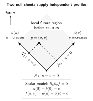
Two transverse initial null sheets supply data to a local future region. Dashed characteristics connect a point to both branches. The scalar model $f_{uv}=0$ gives $f=a(u)+b(v)-c$ when $a(0)=b(0)=c$. Screen directions are suppressed. The schematic illustrates compatibility, not the full Einstein free-data count.

The relevant theorem is deliberately local and gauge fixed.

Statement. In a standard harmonic-coordinate patch, let two smooth null hypersurfaces intersect transversely in a smooth spacelike corner. Prescribe smooth symmetric positive-definite unit-determinant screen data $h_{AB}$ on their union, with a common restriction at the corner, together with the smooth corner functions needed to fix the area scale, its first null derivatives, cross-normalization, and remaining coordinate data. If the null constraints and corner compatibility conditions hold, then a sufficiently small quadrant neighborhood of the corner admits a unique smooth Lorentzian metric in that fixed gauge solving the vacuum Einstein equations and inducing those data. Smooth parameter families of admissible data give smooth parameter families of solutions.

The hypotheses doing real work are:

• the two initial hypersurfaces are smooth, null, and transverse;
• their intersection is a regular orientable spacelike two-surface, treated in one local chart at a time;
• the screen matrix is smooth, positive definite, and nondegenerate, with its determinant gauge fixed;
• the generator orientation, boost normalization, and harmonic or standard coordinate gauge are fixed;
• the data satisfy every null transport constraint and all corner compatibility relations to the differentiability order claimed;
• the neighborhood is chosen before generator crossing or focal degeneration.

Rendall’s precise vacuum result is Rendall 1990, § 5, pp. 230–234, especially Theorem 3 on p. 233. Its uniqueness is uniqueness of the metric components in the fixed standard coordinates. It is not a claim of global development, caustic avoidance, low-regularity well-posedness, or unrestricted geometric uniqueness. Those sharper results and their modern function spaces belong to Existence Theory for the Characteristic Initial-Value Problem.

Why the hierarchy yields a spacetime

The proof architecture has four steps.

First, harmonic gauge converts the vacuum Einstein equations to a quasilinear wave system for the metric components. The characteristic surfaces remain null for the metric determined by the data. Rendall first proves the model existence and uniqueness result for a quasilinear wave equation on two transverse characteristic hypersurfaces in Rendall 1990, §§ 2–3, pp. 223–229, especially Theorem 1 on p. 226.

Second, on each initial null sheet, the restricted Einstein and gauge equations form a hierarchy of ordinary differential equations. Starting with $h_{AB}$ and the corner functions, this hierarchy constructs the missing metric components and the derivatives needed by the reduced wave system. The calculation succeeds on both sheets only when their values at $S$ are compatible.

Third, the characteristic problem for the reduced wave equations is converted locally to an ordinary Cauchy problem. Local Cauchy existence supplies a reduced solution, and domain-of-dependence uniqueness forces it to induce the original data on both null sheets.

Fourth, the harmonic gauge quantities and unsolved Einstein components obey a homogeneous subsidiary system by the contracted Bianchi identity. They vanish on the initial sheets because the transport constraints were imposed, so uniqueness makes them vanish in the local development. The reduced solution is therefore a solution of the full vacuum equations.

This outline explains why constraint-compatible data are indispensable. It does not replace the estimates controlling regularity and continuous dependence.

Independent corner check and failure modes

Take flat spacetime in null Cartesian coordinates,

$$ds^2=-2\,du\,dv+dy^2+dz^2.$$

The sheets $u=0$ and $v=0$ intersect in the spacelike $(y,z)$ plane. Their conformal screen data are both $\delta_{AB}$, both expansions and shears vanish, the cross-normalization is $-1$, and the normal-bundle connection vanishes. Every transport equation preserves these constant values, reconstructing Minkowski space.

Now keep unit determinant but prescribe $\delta_{AB}$ from $\mathcal N_1$ and $\operatorname{diag}(e^{2a},e^{-2a})$ from $\mathcal N_2$ at $S$, with $a\ne0$. No continuous spacetime metric can induce both. Each sheet separately carries smooth-looking data, but the pair is inadmissible because the corner metric is duplicated inconsistently.

A single null cone has a different issue: at its vertex the screen degenerates, so the transverse-corner theorem does not apply without separate vertex regularity analysis. Likewise, even admissible smooth data cease to support this chart after a caustic. The spacetime may remain smooth while the generator labels fail.

Exercises

For the Minkowski null planes above, apply a constant boost $\ell'=c\ell$, $n'=c^{-1}n$. Which corner data change, and why does the local spacetime remain the same?

Solution

The screen metric $\delta_{AB}$ is unchanged. Both shears remain zero. The expansions transform with opposite weights,

$$\theta_{(\ell')}=c\,\theta_{(\ell)}=0, \qquad \theta_{(n')}=c^{-1}\theta_{(n)}=0,$$

and the cross-normalization remains $\ell'\cdot n'=-1$. Because $c$ is constant on the screen, the normal-bundle connection also remains zero.

The component representation of the generator parameters changes, but the conformal data, compatibility conditions, and reconstructed metric do not. If the two sheets were rescaled independently without matching their product at $S$, the corner cross-normalization would be inconsistent; that would be a data error rather than a new solution.

References

• Rendall, Alan D. “Reduction of the Characteristic Initial Value Problem to the Cauchy Problem and Its Applications to the Einstein Equations.” Proceedings of the Royal Society of London A 427, no. 1872 (1990): 221–239. doi:10.1098/rspa.1990.0009.
• Winicour, Jeffrey. “Characteristic Evolution and Matching.” Living Reviews in Relativity 15 (2012): article 2. arXiv:0810.1903. doi:10.12942/lrr-2012-2.