Boundary Data and Constraint Preservation in Einstein Evolution

An Einstein initial-boundary value problem is not obtained by evolving all ten metric components as waves and assigning ten arbitrary boundary functions. The Cauchy data obey constraints; a hyperbolic reduction introduces gauge conditions and a subsidiary constraint system; the boundary admits data only for incoming characteristic combinations; and the boundary data must agree with the initial data at their corner. Well-posedness belongs to this complete reduced system, not to the principal wave operator viewed in isolation.

Required background. The Gibbons–Hawking–York Boundary Term supplies the distinction between variational and evolution boundary data, while PDEs and Green Functions for Gravitation supplies hyperbolic reductions, characteristic fields, and energy estimates.

Helpful background. The Einstein Equation supplies the constraints; Hypersurface Normals and Tangential Projectors supplies initial and boundary geometry; Formulations of General Relativity orients the volume; and Causality and Global Structure supplies domains of dependence.

Five coupled layers of data

Let $S_0$ be a spacelike initial hypersurface with boundary $C$, and let the timelike boundary $\mathcal T$ meet it at $C$. A continuum Einstein IBVP must specify or solve for five layers:

1. Initial geometry: $(\gamma_{ij},K_{ij})$ satisfying the Hamiltonian and momentum constraints, plus compatible matter data.
2. Gauge reduction: coordinate, frame, or gauge-source functions that turn Einstein’s equations into a strongly or symmetrically hyperbolic system.
3. Physical incoming data: typically two radiative combinations, although their exact form depends on the reduction and boundary frame.
4. Gauge and constraint boundary data: conditions that control incoming gauge fields and prevent incoming violations of the subsidiary system.
5. Corner compatibility: equality of the initial and boundary traces and of the time derivatives required by the target regularity.

None can be chosen after the others without a compatibility check. In particular, “fix the boundary metric” is a variational statement; its conversion into admissible incoming fields for a hyperbolic formulation is an additional analytic problem.

Generalized harmonic example

In generalized harmonic gauge define

$$C^\mu=\Gamma^\mu-H^\mu,$$

where $\Gamma^\mu=g^{\rho\sigma}\Gamma^\mu{}_{\rho\sigma}$ and $H^\mu$ are prescribed gauge sources, taken here as functions of coordinates and metric but not metric derivatives. Thus the coordinate equation is $\Box_gx^\mu=-H^\mu$; a source defined instead by $\Box_gx^\mu$ has the opposite sign. The reduced vacuum equations have principal part

$$g^{\rho\sigma}\partial_\rho\partial_\sigma g_{\mu\nu} =\text{lower-order terms}.$$

The reduction is equivalent to Einstein’s equation only when $C^\mu=0$. The Bianchi identity gives a homogeneous subsidiary equation of the schematic form

$$\Box_g C^\mu+R^\mu{}_\nu C^\nu=0.$$

Thus zero initial subsidiary data, including the initial normal derivative of $C^\mu$, remain zero when a uniqueness estimate holds and the boundary supplies homogeneous data for every incoming subsidiary field. Nonzero prescribed subsidiary data can inject constraint violations, even when bounded. Boundary values imposed independently on all $g_{\mu\nu}$ need not imply that condition.

For an outward unit spacelike normal $s^a$ and a future unit timelike boundary vector $T^a$ orthogonal to $s^a$, the null directions

$$K^a=T^a+s^a, \qquad L^a=T^a-s^a$$

are outgoing from and incoming to the computational region, respectively, for this convention. Sommerfeld-type data act on derivatives along an outgoing null direction in such a way that the corresponding incoming characteristic amplitude is controlled. The terminology must always be tied to the chosen normal and boundary matrix.

The figure connects this orientation to admissible data and to the logic of the analysis. Follow the solid $L^a$ arrow into the domain, then read downward: the three input boxes show the generalized-harmonic $2+4+4$ count, whereas the final three boxes separate claims that require distinct arguments and hypotheses.

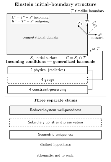
The spacetime cross-section fixes the boundary orientation: $T^a$ is future directed along the timelike wall and $s^a$ points outward, so $K^a=T^a+s^a$ is outgoing and $L^a=T^a-s^a$ is incoming. One common generalized-harmonic hierarchy organizes ten conditions on incoming characteristic fields as two physical, four gauge, and four constraint-preserving conditions; the $2+4+4$ split is formulation-specific. Reduced-system well-posedness, preservation of the subsidiary constraints, and geometric uniqueness are separate statements with separate hypotheses. Transverse directions are suppressed; the figure is schematic and not to scale.

What a well-posed result actually states

For the linear constant-coefficient model, strong well-posedness means an estimate of the form

$$\begin{aligned} \|U(t)\|_{H^m(\Sigma)}^2 +\int_0^t\|U\|_{H^m(\partial\Sigma)}^2\,d\tau &\le C_t \left( \|U(0)\|_{H^m}^2+\int_0^t\|F\|_{H^m}^2d\tau\right)\\ &\quad+C_t\int_0^t\|q\|_{H^m(\partial\Sigma)}^2\,d\tau. \end{aligned}$$

with any derivative shifts stated precisely. The boundary norm is essential: an interior estimate alone does not control the trace needed for a quasilinear iteration.

Kreiss, Reula, Sarbach, and Winicour prove strong well-posedness for a class of half-space harmonic Einstein boundary conditions when specified coefficient matrices have real negative eigenvalues, and extend the result locally to the quasilinear problem, in Kreiss et al. 2007, Theorem 3 and following discussion, pp. 8–10, PDF. This is a named formulation with a structured, sequential set of boundary conditions—not a theorem for arbitrary metric Dirichlet data.

Friedrich and Nagy’s frame formulation provides a complementary result. Given smooth vacuum initial data, their smooth boundary and gauge data, and compatibility to every order, their theorem produces a local-in-time solution on the domain of dependence. The local geometric-uniqueness conclusion in their theorem additionally requires constant boundary mean curvature $\chi=\chi_0$ and vanishing boundary gauge source $F=0$ on $\mathcal T$; it is not part of the unrestricted existence statement. See Friedrich and Nagy 1999, Definition 7.2, Definition 7.3, and Theorem 8.1, pp. 650–652.

Constraint preservation is a separate implication

The logical proof has two stages:

1. solve the reduced hyperbolic IBVP and obtain an energy estimate;
2. show that its gauge and geometric constraints satisfy a homogeneous subsidiary IBVP with zero initial and incoming boundary data.

Uniqueness for the subsidiary problem then gives $C=0$, so the reduced solution solves Einstein’s equation. A stable main system with an uncontrolled subsidiary boundary mode can remain numerically bounded while converging to a solution of the wrong reduced equations.

Independent characteristic count

For ten decoupled scalar waves on a fixed half-space, each field has one incoming and one outgoing normal characteristic combination, so ten scalar boundary conditions are needed. Einstein’s ten wave equations are not ten independent physical fields: four incoming combinations must enforce harmonic constraints, four are associated with coordinate/gauge control, and two encode physical polarizations in a common hierarchical construction. The precise assignment changes with formulation, but the total incoming count does not license ten arbitrary component values.

Common pitfalls

Hyperbolicity of the bulk equations is insufficient. The boundary symbol and its estimate determine whether the IBVP is well posed.

Constraint-preserving conditions do not fix all incoming data. Physical and gauge incoming modes still need admissible prescriptions.

Local existence is not unrestricted geometric uniqueness. Gauge source choices and boundary identification must be included in the theorem’s claim.

Exercise: arbitrary Dirichlet data

Suppose the reduced harmonic equations are solved with arbitrary prescribed $g_{\mu\nu}|_{\mathcal T}$. Explain why constraint-satisfying initial data alone do not ensure an Einstein solution.

Solution

The harmonic constraints satisfy a homogeneous wave equation in the bulk, but their normal derivatives at $\mathcal T$ are combinations of derivatives of the prescribed metric values. Generic componentwise Dirichlet data induce nonzero incoming boundary data for $C^\mu$. A homogeneous subsidiary equation with zero initial data and nonzero boundary data has a nonzero solution, so the reduced metric generally has $C^\mu\ne0$ and does not satisfy the unreduced Einstein equation. One must replace or organize four boundary combinations so that all incoming constraint modes vanish or are consistently controlled.

References

• Friedrich, Helmut, and Gabriel Nagy. “The Initial Boundary Value Problem for Einstein’s Vacuum Field Equation.” Communications in Mathematical Physics 201 (1999): 619–655. DOI.
• Kreiss, Heinz-Otto, Oscar Reula, Olivier Sarbach, and Jeffrey Winicour. “Well-Posed Initial-Boundary Value Problem for the Harmonic Einstein Equations Using Energy Estimates.” Classical and Quantum Gravity 24, no. 23 (2007): 5973–5984. DOI; Open PDF.