Hyperboloidal Slices

A hyperboloidal slice is spacelike in the physical spacetime but approaches an outgoing null hypersurface asymptotically, so its conformal completion meets future null infinity in a spacelike two-surface. It therefore combines a Cauchy-like evolution direction with direct access to radiation at $\mathscr I^+$. The slice does not become physically null: its asymptotic tilt and the conformal compression must be analyzed separately.

Required background. The Riemann Curvature Tensor supplies the geometric conventions used in the conformal completion.

Helpful background. We use The Einstein Equation, Hypersurface Normals and Tangential Projectors, Formulations of General Relativity, and Causality and Global Structure.

Spacelike slices that approach an outgoing light cone

In an asymptotically flat physical spacetime $\widetilde g$, a future hyperboloidal time function $\tau$ has spacelike level sets whose outgoing end approaches constant retarded time. In spherical Minkowski coordinates, write

$$d\widetilde s^2=-dt^2+dr^2+r^2d\omega_2^2$$

and choose the height function

$$t=\tau+\sqrt{r^2+a^2}, \qquad a\gt 0.$$

At large $r$,

$$t-r=\tau+\frac{a^2}{\sqrt{r^2+a^2}+r}\longrightarrow\tau.$$

Thus each level set approaches the outgoing null hypersurface $u=t-r=\tau$. Yet its slope obeys

$$\left|\frac{dt}{dr}\right| =\frac{r}{\sqrt{r^2+a^2}}\lt 1$$

at every finite $r$, so the slice is strictly spacelike in the physical metric. Ordinary constant-$t$ slices instead run toward spatial infinity, not a cut of $\mathscr I^+$.

The future-directed physical unit normal and induced metric are

$$\widetilde n^\mu =\left(\frac{\sqrt{r^2+a^2}}a,\frac ra,0,0\right),$$ $$d\widetilde\ell^2 =\frac{a^2}{r^2+a^2}\,dr^2+r^2d\omega_2^2.$$

Both formulas can be checked directly: $\widetilde n^2=-1$, and the radial coefficient equals $1-(dt/dr)^2\gt 0$. With the site convention

$$\widetilde K_{ij} =-\widetilde h_i{}^\mu\widetilde h_j{}^\nu \widetilde\nabla_\mu\widetilde n_\nu,$$

the hyperboloid has

$$\widetilde K_{ij}=-\frac1a\widetilde h_{ij}, \qquad \widetilde K=-\frac3a.$$

It is therefore constant-mean-curvature data with negative mean curvature for the future normal in the site’s sign convention. Andersson discusses these Minkowski hyperboloids and their conformal endpoints in Andersson 2002, § 3, pp. 185–187.

Compactifying the radial end

Choose the dimensionless conformal factor

$$\Omega=\frac{a}{\sqrt{r^2+a^2}}, \qquad r=\frac{a\sqrt{1-\Omega^2}}{\Omega}.$$

For $r\gt0$, the new radial coordinate has $0\lt\Omega\lt1$, and future null infinity is at $\Omega=0$. It is a useful chart near infinity, not a regular radial coordinate at the center $r=0$, where $d\Omega/dr=0$ and spherical angular coordinates also degenerate. The apparent pole at $\Omega=1$ in the radial metric below is therefore a coordinate issue at the center. Moving outward along the slice means decreasing $\Omega$; consequently the outward co-orientation of its compact boundary is opposite to $d\Omega$, which points toward increasing $\Omega$.

The diagram separates physical spacelikeness from conformal nullness. In panel (a), compare the hyperboloid with its outgoing null asymptote; in panel (b), follow the spacelike slice to its two-sphere cut and read the transverse arrow only as the boundary co-orientation.

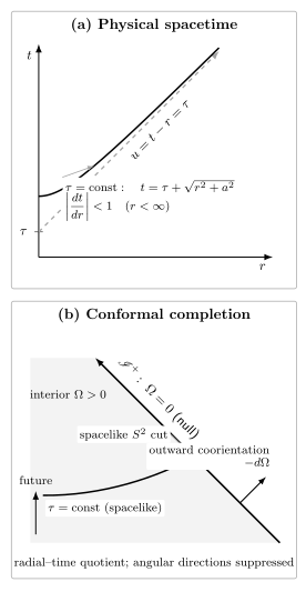
A finite-radius hyperboloidal slice remains spacelike because $\lvert dt/dr\rvert\lt 1$ while approaching the outgoing null hypersurface $u=t-r=\tau$. After conformal compactification, the same $\tau=\mathrm{const}$ slice reaches the null boundary $\mathscr I^+$ at a spacelike $S^2$ cut. The shaded interior has $\Omega\gt 0$, and the transverse arrow denotes the outward co-orientation $-d\Omega$, not a metric-raised normal vector. Schematic and not to scale.

Multiplying the induced metric by $\Omega^2$ gives

$$d\ell^2 =\Omega^2d\widetilde\ell^2 =\frac{a^2}{1-\Omega^2}\,d\Omega^2 +a^2(1-\Omega^2)d\omega_2^2.$$

This metric is positive definite and smooth at $\Omega=0$; the boundary cut is a round two-sphere of radius $a$ in this conformal representative. The physical proper distance to the end still diverges logarithmically. Compactification changes the metric representative and coordinate range, not the physical distance.

The full unphysical metric in $(\tau,\Omega)$ coordinates is

$$ds^2=\Omega^2d\widetilde s^2 =-\Omega^2d\tau^2+2a\,d\tau\,d\Omega +\frac{a^2}{1-\Omega^2}d\Omega^2 +a^2(1-\Omega^2)d\omega_2^2.$$

It remains nondegenerate at $\Omega=0$. Inverting its $(\tau,\Omega)$ block gives

$$g^{\Omega\Omega} =\frac{\Omega^2(1-\Omega^2)}{a^2},$$

so $(\nabla\Omega)^2=0$ at the boundary. The endpoint is therefore null as a spacetime boundary even though its intersection with each hyperboloidal slice is a spacelike two-sphere.

What hyperboloidal does and does not mean

“Hyperboloidal” describes asymptotic causal behavior, not necessarily exact hyperbolic shape or constant mean curvature. Many useful slices have a standard interior and become hyperboloidal only in an exterior layer. Conversely, a spacelike surface merely extending to large radius is not hyperboloidal unless its retarded-time limit is finite and its conformal completion is regular.

A hyperboloidal hypersurface is also not generally a global Cauchy surface for the entire asymptotically flat spacetime: it omits spatial infinity and may cover only the future domain relevant to its cut of $\mathscr I^+$. Zenginoğlu emphasizes this domain distinction in Zenginoğlu 2008, § 1, pp. 1–2.

Exercises

For the Minkowski hyperboloid above, verify its unit normal, compute its mean curvature with the site’s sign, and show that the conformal induced metric has a regular positive limit at $\Omega=0$.

Solution

The stated normal satisfies $-({r^2+a^2})/a^2+r^2/a^2=-1$ and is future directed. In Cartesian spatial coordinates it is $\widetilde n=(\sqrt{r^2+a^2}/a,x^i/a)$, so tangential projection of $\widetilde\nabla_i\widetilde n_j$ equals $\widetilde h_{ij}/a$. The leading minus in the definition gives $\widetilde K_{ij}=-\widetilde h_{ij}/a$ and $\widetilde K=-3/a$. Finally, substituting $dr=-a[\Omega^2\sqrt{1-\Omega^2}]^{-1}d\Omega$ gives

$$\Omega^2d\widetilde\ell^2 =\frac{a^2}{1-\Omega^2}d\Omega^2 +a^2(1-\Omega^2)d\omega_2^2,$$

whose radial eigenvalue tends to $a^2$ and whose angular metric tends to $a^2d\omega_2^2$.

References

• Andersson, Lars. “Construction of Hyperboloidal Initial Data.” In The Conformal Structure of Spacetimes: Geometry, Analysis, Numerics, edited by Jörg Frauendiener and Helmut Friedrich, Lecture Notes in Physics 604, 183–194. Springer, 2002. arXiv:gr-qc/0205083.
• Zenginoğlu, Anıl. “Hyperboloidal Evolution with the Einstein Equations.” Classical and Quantum Gravity 25 (2008): 195025. DOI. Open PDF.