Spacelike Foliations and Evolution Vectors

A spacelike foliation replaces one four-dimensional field equation by a family of spatial problems tied together by an evolution rule. The coordinate time flow then has two geometrically distinct parts: the lapse advances a slice in its future-normal direction, while the shift relabels points tangentially within the slice. Neither is an additional gravitational degree of freedom.

Required background. Hypersurface Normals and Tangential Projectors supplies the induced metric and spatial projector, while The Einstein Equation supplies the covariant dynamics that will be decomposed.

Helpful background. The Gibbons-Hawking-York Boundary Term explains why the normal derivative of the spatial metric is also the natural boundary datum in the gravitational action.

A time function and its slices

Let $t:\mathcal M\to\mathbb R$ be a smooth time function on a region where its gradient is timelike. Its level sets

$$\Sigma_t=\{p\in\mathcal M:t(p)=\text{constant}\}$$

are spacelike hypersurfaces. Their future-directed unit normal is fixed by

$$\alpha =\left(-g^{\mu\nu}\nabla_\mu t\nabla_\nu t\right)^{-1/2}, \qquad n_\mu=-\alpha\nabla_\mu t, \qquad n^\mu n_\mu=-1,$$

where $t$ is chosen to increase toward the future and $\alpha\gt0$. The spatial metric and mixed projector are

$$\gamma_{\mu\nu}=g_{\mu\nu}+n_\mu n_\nu, \qquad \gamma^\mu{}_\nu=\delta^\mu{}_\nu+n^\mu n_\nu.$$

They annihilate the normal and restrict to a positive-definite metric on each $\Sigma_t$. A tensor is spatial when projection on every index leaves it unchanged.

Because $n^\mu\nabla_\mu t=1/\alpha$, the vector

$$m^\mu\equiv\alpha n^\mu$$

satisfies $m^\mu\nabla_\mu t=1$. Flowing by coordinate parameter $dt$ along $m^\mu$ therefore reaches the next level set, and the proper time measured by the normal observers is $d\tau=\alpha\,dt$. Spatial variation of the lapse accelerates those observers:

$$a_i\equiv\gamma_i{}^\mu n^\nu\nabla_\nu n_\mu=D_i\ln\alpha.$$

Thus a lapse constant on each slice gives geodesic normal curves, although those curves can still focus and cease to furnish a good foliation.

Normal advance and tangential relabeling

Choose spatial coordinates $x^i$ on one slice and extend them through the foliation. The coordinate time vector $t^\mu=(\partial_t)^\mu$ also satisfies $t^\mu\nabla_\mu t=1$. Consequently its difference from $m^\mu$ is tangent to the slices:

$$t^\mu=\alpha n^\mu+\beta^\mu, \qquad n_\mu\beta^\mu=0.$$

This is the lapse-shift split. The lapse controls the normal separation of neighboring slices. The shift $\beta^i$ controls which point on $\Sigma_{t+dt}$ inherits the same spatial coordinate label as a point on $\Sigma_t$.

The vector triangle below makes the two operations distinct: follow the normal arrow to advance the geometry, then follow the tangential arrow to the point carrying the same coordinate label.

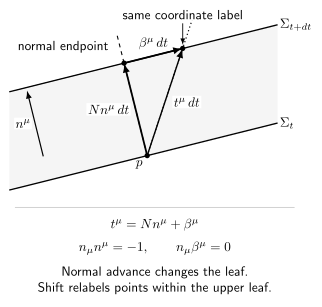
A coordinate-time displacement is the sum of normal proper advance $Nn\,dt$ and tangential coordinate shift $\beta\,dt$; the figure’s $N$ denotes the lapse $\alpha$ used here. A coordinate line is normal only when the shift vanishes. Schematic and not to scale.

For a spatial tensor $T$, the derivative representing normal evolution is

$$\partial_\perp T\equiv(\partial_t-\mathcal L_\beta)T =\alpha\,\operatorname{proj}_{\Sigma}(\mathcal L_nT).$$

Here every free index on the right is projected onto the slice. This qualification matters for contravariant indices: for a spatial vector $X$, $\mathcal L_{\alpha n}X=\alpha\mathcal L_nX-X(\alpha)n$ before projection. The extra term is normal and disappears after projection. For the spatial metric with both indices pulled back to the slice, the familiar shorthand $\partial_\perp\gamma_{ij}=\alpha(\mathcal L_n\gamma)_{ij}$ is therefore valid.

The coordinate lines $x^i=\text{constant}$ need not be timelike. Indeed,

$$g_{\mu\nu}t^\mu t^\nu =-\alpha^2+\gamma_{ij}\beta^i\beta^j.$$

A large shift may make $t^\mu$ spacelike without changing the fact that the slices themselves are spacelike. This is motion of labels, not superluminal motion of matter.

The intrinsic and extrinsic gravitational data on a slice are $(\gamma_{ij},K_{ij})$. The lapse and shift choose how those data are represented during evolution. With the convention used throughout this volume,

$$K_{ij}=-\frac12\mathcal L_n\gamma_{ij},$$

so later pages will obtain $\partial_\perp\gamma_{ij}=-2\alpha K_{ij}$. The six components of $\gamma_{ij}$ and six of $K_{ij}$ are restricted by four Einstein constraints; lapse and shift do not supply four missing physical modes.

These geometric constructions and the adapted-coordinate split are developed in Gourgoulhon 2007, §§3.2.2–3.3.5, pp. 40–46 and §§4.2.1–4.2.2, pp. 54–57, PDF.

Two foliations of Minkowski spacetime

In inertial coordinates,

$$ds^2=-dT^2+dX^2+dY^2+dZ^2,$$

take $t=T$ and $x^i=(X,Y,Z)$. Then

$$\alpha=1, \qquad \beta^i=0, \qquad n=\partial_T, \qquad \gamma_{ij}=\delta_{ij}.$$

The normal observers and coordinate threads coincide. A moving grid gives a different split of the same foliation. Set $t=T$ and $y=X-vT$. Since $X=y+vt$,

$$ds^2=-(1-v^2)dt^2+2v\,dt\,dy+dy^2+dY^2+dZ^2.$$

The slices are still the inertial hyperplanes, with $\alpha=1$ and Euclidean $\gamma_{ij}$, but $\beta^y=v$. The normal is $n=\partial_t-v\partial_y=\partial_T$. Even for $\lvert v\rvert>1$, when $\partial_t$ is spacelike, the hypersurfaces and their future normal remain perfectly regular.

For a genuinely different foliation, use Milne coordinates inside the future light cone:

$$T=\tau\cosh\chi, \qquad R=\tau\sinh\chi,$$

which give

$$ds^2=-d\tau^2+\tau^2 \left(d\chi^2+\sinh^2\chi\,d\Omega^2\right).$$

Here $\alpha=1$, $\beta^i=0$, and $n=\partial_\tau$, but the slices are expanding hyperboloids rather than flat hyperplanes. Their nonzero extrinsic curvature does not signal spacetime curvature: both descriptions cover regions of Minkowski spacetime. This pair will provide a recurring sign check for the rest of the chapter.

Common pitfalls

A foliation is not a coordinate system. The time function determines the slices; the shift additionally determines how spatial labels are threaded between them.

The coordinate time vector need not be timelike. Spacelikeness of $\partial_t$ caused by a large shift does not make the level sets of $t$ nonspacelike.

Lapse and shift are not freely specifiable physical data. They express a gauge choice. The constraint-satisfying pair $(\gamma_{ij},K_{ij})$ and matter data determine the physical initial-value problem up to gauge.

Exercise: a moving Cartesian grid

For the moving-grid metric above, compute $g(\partial_t,\partial_t)$, identify the normal vector, and show that normal observers measure one unit of proper time per unit $dt$ even when $\lvert v\rvert>1$.

Solution

The coordinate time vector has squared norm

$$g(\partial_t,\partial_t)=g_{tt}=-(1-v^2).$$

It is spacelike for $\lvert v\rvert>1$. From $\alpha=1$ and $\beta=v\partial_y$,

$$n=\frac{1}{\alpha}(\partial_t-\beta) =\partial_t-v\partial_y =\partial_T.$$

Therefore $g(n,n)=-1$, and a displacement normal to the slices is $d\tau=\alpha\,dt=dt$. The superluminal-looking coordinate thread is only a rapid relabeling; the normal observers remain ordinary inertial observers.

References

• Gourgoulhon, Éric. 3+1 Formalism and Bases of Numerical Relativity. Lecture notes, arXiv:gr-qc/0703035v1 (2007). arXiv.