Spin Coefficients and Null-Congruence Geometry

Spin coefficients are the components of the Levi-Civita connection in a null tetrad. Eight of them directly describe how the two null directions bend and how their transverse screens expand, shear, and twist; four more supply the boost-spin connection needed to differentiate weighted components. Their signs are not intrinsic to their Greek names, so this page defines every coefficient by contraction before assigning a geometric interpretation.

Required background. Frames, coframes, and anholonomy supplies the frame connection; The Riemann curvature tensor relates its derivatives to curvature; The Einstein equation identifies the Ricci focusing terms.

Helpful background. Hypersurface normals and tangential projectors supplies transverse projectors; Timelike congruences and spatial projection provides the expansion–shear–twist decomposition that has a null analogue here.

Connection components of the two null directions

Assume the ordered tetrad and normalization

$$(\ell,n,m,\bar m),\qquad \ell\cdot n=-1,\qquad m\cdot\bar m=1,$$

with all other inner products zero. Define the eight properly weighted coefficients by

$$\begin{aligned} \kappa&=-\ell^a m^b\nabla_a\ell_b, &\kappa'&=-\bar m^a n^b\nabla_b n_a,\\ \rho&=-m^a\bar m^b\nabla_b\ell_a, &\rho'&=-m^a\bar m^b\nabla_a n_b,\\ \sigma&=-m^a m^b\nabla_a\ell_b, &\sigma'&=-\bar m^a\bar m^b\nabla_b n_a,\\ \tau&=-m^a n^b\nabla_b\ell_a, &\tau'&=-\ell^a\bar m^b\nabla_a n_b. \end{aligned}$$

The leading minus signs are part of this site’s $(-,+,+,+)$ convention. They make these coefficients agree numerically with the coefficients in Andersson et al. 2022, §3.1, Definition 3.1, equations (3.1a)–(3.1d), PDF after the source metric, which has the opposite signature and null normalization, is multiplied by $-1$. This is a contraction-by-contraction translation, not a rule that every Newman–Penrose scalar always receives one minus sign.

The remaining four coefficients are

$$\begin{aligned} \beta={}&\frac12 m^a\bar m^b\nabla_a m_b +\frac12\ell^a m^b\nabla_b n_a,\\ \beta'={}&-\frac12\bar m^a\bar m^b\nabla_b m_a -\frac12\ell^a\bar m^b\nabla_b n_a,\\ \epsilon={}&\frac12\ell^a\bar m^b\nabla_a m_b +\frac12\ell^a\ell^b\nabla_b n_a,\\ \epsilon'={}&-\frac12\bar m^a n^b\nabla_b m_a -\frac12\ell^a n^b\nabla_b n_a. \end{aligned}$$

Unlike the first eight, these four transform inhomogeneously under a local boost or spin. They are therefore connection components rather than properly weighted scalars.

The prime is part of a coefficient’s name; it is neither a derivative nor complex conjugation. The bar denotes complex conjugation. There are twelve complex coefficients because a metric-compatible connection in four dimensions has $4\times6=24$ real components. The vector $n$ in this chapter is the second null leg, not the unit timelike normal of the 3+1 chapters.

Optical meaning and weights

The screen metric orthogonal to $\ell^a$ and $n^a$ is

$$q_{ab}=m_a\bar m_b+\bar m_a m_b.$$

Projecting $\nabla_b\ell_a$ twice with $q_a{}^b$ produces the optical tensor. It is important to distinguish the full area expansion used elsewhere in this volume from the averaged Newman–Penrose expansion. With the definitions above,

$$\theta_{(\ell)} =q^{ab}\nabla_b\ell_a =-2\operatorname{Re}\rho, \qquad \theta_{\mathrm{NP}} =\frac12\theta_{(\ell)} =-\operatorname{Re}\rho.$$

Here $\theta_{(\ell)}=\ell(\ln\sqrt q)$ is the fractional rate of change of a transported infinitesimal screen-area element, whereas $\theta_{\mathrm{NP}}$ is the average per transverse dimension. For a twisting congruence, the screen planes need not form a family of surfaces; the area statement concerns a transported pencil of rays.

More explicitly, in the oriented real screen basis with $m=(e_2+i e_3)/\sqrt2$, put $B_{AB}=e_A{}^a e_B{}^b\nabla_b\ell_a$, for $A,B=2,3$. Its decomposition is

$$B_{AB}= \begin{pmatrix} \theta_{(\ell)}/2+s_1&s_2+w\\ s_2-w&\theta_{(\ell)}/2-s_1 \end{pmatrix}, \qquad \rho=-\frac12\theta_{(\ell)}+iw, \qquad \sigma=-s_1-i s_2.$$

The trace changes the area, the symmetric trace-free part changes a small circle into an ellipse, and the antisymmetric part rotates neighboring rays relative to a transported screen. In particular, the squared shear and twist tensors are $2|\sigma|^2$ and $2(\operatorname{Im}\rho)^2$. This fixes the otherwise easy-to-miss factors of two in Raychaudhuri’s equation.

Follow the marked ray in each panel: changing the circle’s area, changing its shape, and rotating its labels are three distinguishable operations.

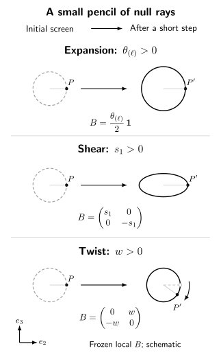
The three parts of the optical tensor act differently on an infinitesimal pencil of null rays. The marked ray $P$ moves to $P'$. Each panel isolates one constant local part of $B$ for a short positive affine step; the rightward and upward axes are $e_2$ and $e_3$. Positive $w$ rotates the marker clockwise with the matrix convention shown. This is a schematic frozen-coefficient comparison, not an integrated solution of the Sachs equations.

The acceleration has the exact decomposition

$$\ell^b\nabla_b\ell^a =2\operatorname{Re}\epsilon\,\ell^a -\bar\kappa m^a-\kappa\bar m^a.$$

Thus $\kappa=0$ makes the rays geodesic, and $\operatorname{Re}\epsilon=0$ also makes their parameter affine. $\operatorname{Im}\epsilon$ instead describes the screen’s spin rotation along the ray. Primed coefficients give the corresponding geometry for $n$.

Under $\ell\mapsto A\ell$ and $m\mapsto e^{i\chi}m$, the weights $(b,s)$ are

$$\begin{array}{c|cccccccc} \eta&\kappa&\sigma&\rho&\tau&\kappa'&\sigma'&\rho'&\tau'\\ \hline (b,s)&(2,1)&(1,2)&(1,0)&(0,1)&(-2,-1)&(-1,-2)&(-1,0)&(0,-1). \end{array}$$

For example, $\rho\mapsto A\rho$ and $\sigma\mapsto A e^{2i\chi}\sigma$. Derivatives of $A$ or $\chi$ cancel from these eight contractions because they multiply vanishing tetrad inner products. The same cancellation does not occur for $\epsilon,\epsilon',\beta,\beta'$.

A flat-space check

In Minkowski spacetime with spherical coordinates, take

$$\ell=\frac{\partial_t+\partial_r}{\sqrt2},\qquad n=\frac{\partial_t-\partial_r}{\sqrt2},\qquad m=\frac1{\sqrt2 r}\left(\partial_\theta+i\csc\theta\,\partial_\phi\right).$$

Direct evaluation with the spherical-coordinate Christoffel symbols gives

$$\kappa=\sigma=\tau=0, \qquad \rho=-\frac1{\sqrt2 r},$$

and, for the ingoing direction, $\kappa'=\sigma'=\tau'=0$ and $\rho'=1/(\sqrt2 r)$. Thus $\theta_{\mathrm{NP}}=1/(\sqrt2 r)$, while the screen-area expansion is $\theta_{(\ell)}=\sqrt2/r$. Indeed, $\ell(\ln r^2)=\sqrt2/r$. Flat spacetime does not imply vanishing spin coefficients: a curvilinear or accelerating tetrad can have a nonzero connection even when its curvature is zero. The displayed $m$ is also singular at the polar axis; overlapping angular frames are required there.

The twelve conventional unprimed Greek names found in older Newman–Penrose sources package the same connection data with signature-dependent identifications. Equation (27) of Gómez López and Quiroga 2017, §II.B, p. 3, PDF is a useful comparison only after translating both its metric dyad and its rotation coefficients.

Exercises

Compute $\rho$ for the outgoing Minkowski tetrad above and check its boost weight by replacing $\ell$ with $A\ell$ and $n$ with $A^{-1}n$, where $A$ is a positive constant.

Solution

The angular connection components give $\nabla_\theta\ell_\theta=r/\sqrt2$ and $\nabla_\phi\ell_\phi=r\sin^2\theta/\sqrt2$. Contracting with $m^a\bar m^b$ adds two equal contributions, so $m^a\bar m^b\nabla_b\ell_a=1/(\sqrt2 r)$. The defining minus sign yields $\rho=-1/(\sqrt2 r)$. For constant $A$, the lowered vector $\ell_a$ contributes $A$, while $m$ and $\bar m$ are unchanged, hence $\rho\mapsto A\rho$. Its boost weight is therefore $b=1$, in agreement with the table.

References

• Andersson, Lars, Thomas Bäckdahl, Pieter Blue, and Siyuan Ma. “Nonlinear Radiation Gauge for Near Kerr Spacetimes.” Communications in Mathematical Physics 396 (2022): 45–90. DOI.
• Gómez López, L. A., and G. D. Quiroga. “Asymptotic Structure of Spacetime and the Newman–Penrose Formalism: A Brief Review.” arXiv:1711.11381v1 (2017). arXiv.