Hellings–Downs Correlations

Scrollable formula. Use Left and Right arrow keys to reveal hidden content.

Scrollable table. Use Left and Right arrow keys to reveal additional columns.

Scrollable figure. Use Left and Right arrow keys to inspect hidden content.

An isotropic, stationary, unpolarized tensor background produces a distinctive angular correlation between timing residuals from different pulsars. The Hellings–Downs curve is neither a fitted spectral slope nor a correlation of pulse profiles; it is the sky-averaged product of two one-way gravitational-wave antenna responses. Its non-monopolar shape distinguishes tensor gravitational radiation from a common clock error and helps separate it from Solar-System ephemeris error.

Helpful background. Earth Terms, Pulsar Terms, and Antenna Response derives the one-way response. Stochastic Cross-Correlation defines random-field cross-correlation.

The overlap integral

For distinct pulsars $a$ and $b$ , the Earth-term cross-spectrum of an isotropic tensor background has the form

\left\langle\widetilde r_a(f) \widetilde r_b^*(f')\right\rangle =\frac12\delta(f-f') \Gamma_{ab}\,P_{\rm gw}(f),

under a one-sided residual-spectrum convention. With $e^A_{ij}e^{B,ij}=2\delta^{AB}$ and the antenna factors defined on the preceding page, the normalized angular factor is

\Gamma_{ab}=\frac{3}{8\pi} \int_{S^2}d\boldsymbol\Omega \sum_{A=+,\times} F_a^A(\boldsymbol\Omega)F_b^A(\boldsymbol\Omega).

To see how geometry enters, put $\mu_a=\boldsymbol\Omega\cdot\boldsymbol p_a$ , $\mu_b=\boldsymbol\Omega\cdot\boldsymbol p_b$ , and $q=\boldsymbol p_a\cdot\boldsymbol p_b$ . The transverse-traceless polarization sum gives the basis-independent integrand

\sum_A F_a^AF_b^A =\frac{2(q-\mu_a\mu_b)^2 -(1-\mu_a^2)(1-\mu_b^2)} {4(1+\mu_a)(1+\mu_b)}.

Align $\boldsymbol p_a$ with the polar axis and place $\boldsymbol p_b$ in the meridian at separation $\zeta$ . Then $\mu_a=\cos\theta$ and $\mu_b=\cos\theta\cos\zeta+\sin\theta\sin\zeta\cos\phi$ . Integrating over $d\boldsymbol\Omega=\sin\theta\,d\theta\,d\phi$ gives

\Gamma_{\rm HD}(\zeta) =\frac12+\frac32x\ln x-\frac14x, \qquad x=\frac{1-\cos\zeta}{2},

where $x\ln x\to0$ as $x\to0$ . The autocorrelation adds a pulsar-term contribution, often written $+\tfrac12\delta_{ab}$ in this normalization. Consequently, the distinct-pulsar zero-separation limit is $1/2$ , while the same-pulsar value is $1$ . Mixing these normalizations is a common factor-of-two error.

The normalization can be checked without the general angular integral. For coincident directions, the integrand reduces to $(1-\mu_a)^2/4$ . Its sky integral is $4\pi/3$ , which becomes $1/2$ after multiplication by $3/(8\pi)$ . This limit assumes large pulsar distances and incoherent pulsar phases; physically nearby pulsars need the full frequency-dependent response Romano and Allen 2024, §§3.1 and 4, questions 1–3.

Useful checks are

\Gamma_{\rm HD}(0)=\frac12, \qquad \Gamma_{\rm HD}(\pi)=\frac14,

with negative correlation at intermediate angles. Hellings and Downs derived the angular signature in the original PTA calculation Hellings and Downs 1983, pp. L39–L42.

Separation	Distinct-pulsar tensor correlation
0°	0.5000
30°	0.2116
60°	−0.0824
90°	−0.1449
120°	−0.0111
150°	0.1697
180°	0.2500

Clock, ephemeris, and tensor patterns

Compare the middle-angle dip in the tensor curve with the simpler controls below. Their overall amplitudes are chosen only to compare shapes; a real analysis fits amplitudes and uses the actual pulsar-pair covariance.

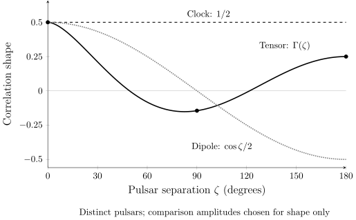
The tensor correlation becomes negative at intermediate pulsar separations and returns to one quarter at 180 degrees, unlike a constant clock correlation or a cosine dipole.

The Hellings–Downs curve for distinct pulsars in an isotropic, unpolarized tensor background differs from monopole and dipole angular patterns. The controls are scaled to $1/2$ at zero separation to compare shapes, not to predict their physical amplitudes. These are analytic curves, with no measured points or same-pulsar autocorrelation term; pulsar phases are assumed incoherent.

A terrestrial time-standard error enters every pulsar with the same sign, producing a monopolar correlation approximately constant in separation. An error in the solar-system barycenter projects along each pulsar direction and produces a dipolar pattern proportional to $\boldsymbol p_a\cdot\boldsymbol p_b$ for an isotropic ephemeris-error vector model.

The Hellings–Downs curve contains quadrupolar and higher multipoles. In the continuous, uniformly weighted sky average, its monopole and dipole moments vanish:

\int_0^1\Gamma_{\rm HD}(x)\,dx=0, \qquad \int_0^1(1-2x)\Gamma_{\rm HD}(x)\,dx=0.

For example, the first identity follows from $\int_0^1x\ln x\,dx=-1/4$ . A positive background power can therefore produce negative correlations at some angles. This orthogonality is lost for a finite, irregular sky distribution with unequal pulsar noise. The likelihood must evaluate the actual array response rather than classify a binned plot by eye.

Process	Leading spatial pattern	Main diagnostic
Clock error	Monopole	Same-sign correlation across the sky
Ephemeris error	Dipole	Correlation tied to pulsar directions and planetary basis
Isotropic tensor background	Hellings–Downs	Characteristic sign-changing angular curve
Uncorrelated common spectrum	None between pulsars	Similar auto-spectra without cross-covariance

Why data points do not lie on a perfect curve

Even a Gaussian isotropic background has realization variance: a finite observation samples only finitely many random temporal modes. Pulsar terms add further fluctuations to pair estimates, and shared pulsars make those estimates correlated. A population dominated by a few bright binaries can introduce additional anisotropy or non-Gaussian fluctuations. None of these effects requires each measured pair to equal the ensemble curve; the joint estimator covariance must describe their scatter.

Therefore a plot of binned correlations is explanatory, while evidence comes from the joint covariance likelihood or a validated frequentist cross-correlation statistic. The noise model, spectral model, timing fit, pulsar selection, and ephemeris are marginalized together.

Evidence through 2026-08-18

The NANOGrav 15-year analysis reports evidence for a common red process with spatial correlations consistent with the Hellings–Downs pattern, using multiple Bayesian and frequentist statistics and noise/ephemeris checks Agazie et al. 2023, §§3–5. Contemporary releases provide independent but differently weighted evidence. The EPTA modern-backend subset gives materially stronger Hellings–Downs support than its longer, heterogeneous span, and adding InPTA is broadly consistent with that result Antoniadis et al. 2023, §§4.2–5, Table 5, Figs. 5–8 and 14. The PPTA full-likelihood Bayes factors do not significantly prefer Hellings–Downs correlations over an uncorrelated process, while a cross-correlation-only statistic gives approximately $2\sigma$ evidence Reardon et al. 2023, §§3.6–3.7 and 5, Figs. 7–8. CPTA reports a $4.6\sigma$ comparison between Hellings–Downs and constant correlation at one frequency near $14\,\mathrm{nHz}$ ; that statistic does not exclude a dipole Xu et al. 2023, §§4–5, Fig. 4, and Appendices A and C.

This supports a nanohertz gravitational-wave background interpretation more strongly than an uncorrelated common-spectrum process. It does not uniquely identify supermassive-black-hole binaries, prove exact isotropy or Gaussianity, or exclude clock/ephemeris contributions at all amplitudes.

Independent checks and failure cases

Inject tensor, monopole, dipole, and uncorrelated processes into the real cadence and recover their model odds and frequentist statistics.
Vary Solar-System ephemerides and explicit ephemeris-perturbation models.
Use leave-one-pulsar and sky-scramble tests while accounting for their nonindependence.
Compare binned estimators with the full covariance likelihood.
Allow anisotropy and alternative polarizations; a changed fit does not automatically invalidate tensor power but tests the isotropic model.
Verify endpoint and normalization conventions in code with analytic pairs.

Review after a new public PTA or IPTA release, a corrected noise/ephemeris model, or an independent analysis that changes the spatial-correlation evidence.

Exercises

1. Right-angle pair. Evaluate the distinct-pulsar Hellings–Downs correlation at $\zeta=90^\circ$ .

Solution

Here $x=(1-0)/2=1/2$ , so

\Gamma_{\rm HD} =\frac12+\frac34\ln\frac12-\frac18 \approx-0.145.

The negative value is an important part of the sign-changing tensor pattern.

2. Two co-located directions. Why is the cross-correlation limit for two distinct pulsars in the same direction $1/2$ , not the autocorrelation value $1$ ?

References

Section titled “References”- Agazie, Gabriella, et al. “The NANOGrav 15-Year Data Set: Evidence for a Gravitational-Wave Background.” Astrophysical Journal Letters 951 (2023): L8. DOI. Open PDF.
- Antoniadis, J., et al. “The Second Data Release from the European Pulsar Timing Array. III. Search for Gravitational Wave Signals.” Astronomy & Astrophysics 678 (2023): A50. DOI. Open PDF.
- Hellings, R. W., and G. S. Downs. “Upper Limits on the Isotropic Gravitational Radiation Background from Pulsar Timing Analysis.” Astrophysical Journal Letters 265 (1983): L39–L42. DOI.
- Reardon, Daniel J., et al. “Search for an Isotropic Gravitational-Wave Background with the Parkes Pulsar Timing Array.” Astrophysical Journal Letters 951 (2023): L6. DOI. Open PDF.
- Romano, Joseph D., and Bruce Allen. “Answers to Frequently Asked Questions about the Pulsar Timing Array Hellings and Downs Curve.” Classical and Quantum Gravity 41 (2024): 175008. DOI. Open PDF.
- Xu, Heng, et al. “Searching for the Nano-Hertz Stochastic Gravitational Wave Background with the Chinese Pulsar Timing Array Data Release I.” Research in Astronomy and Astrophysics 23 (2023): 075024. DOI. Open PDF.