Selection Functions from Injections

A selection function is the probability that the complete search-and-reporting procedure includes a source with specified parameters and data-state conditions. It is not merely a signal-to-noise threshold. Injection campaigns estimate this probability by placing known signals into representative data, running the declared pipeline, and counting recoveries with importance weights that match the target source distribution.

Helpful background. Search-level injection design begins in Injection Campaigns and Search Sensitivity. The threshold whose efficiency is measured must be the one defined in Detection Thresholds and False-Alarm Accounting.

Detection probability and population efficiency

Let $\theta$ denote source parameters and $x$ the detector state, calibration, observing epoch, and other conditions entering the search. For catalog rule $\mathcal S$, define

$$p_{\mathrm{det}}(\theta,x) = \int dd\, \mathbf 1[\mathcal S(d,x)=1]\, p(d\mid\theta,x).$$

Here $d$ denotes the data, $\mathbf1$ is one when the selection rule is satisfied and zero otherwise, and $\int dd$ integrates over all possible data realizations. This probability averages over noise under the declared data model. For a normalized population density $\pi(\theta\mid\Lambda)$, with shape parameters $\Lambda$, and a normalized distribution $p(x)$ of observing states, the selection fraction is

$$\alpha(\Lambda) = \int d\theta\,dx\, p_{\mathrm{det}}(\theta,x) \pi(\theta\mid\Lambda)p(x).$$

Thus $\alpha$ is the fraction of sources expected to be selected, averaged over source properties and observing conditions. The product $\pi(\theta\mid\Lambda)p(x)$ assumes their distributions are independent; use their joint density if the source population changes with observing state. The same source can be detectable in one detector epoch and missed in another. The detector/source-frame transformation, redshift measure, observing time, duty cycle, calibration, waveform content, and pipeline threshold must therefore match the population likelihood in which $\alpha$ is used.

Importance sampling with recovered injections

A two-class example

First consider exact class labels with no measurement error. Let the intrinsic fractions be $f_A=f_B=0.5$ and the detection probabilities be $\epsilon_A=0.2$, $\epsilon_B=0.8$. Of 1000 sources, the expected detected counts are 100 in A and 400 in B. Thus $\alpha=0.5$, while the fractions within the detected sample are $q_A=0.2$, $q_B=0.8$:

$$q_j=\frac{\epsilon_j f_j}{\alpha}, \qquad \alpha=\sum_j\epsilon_j f_j.$$

The figure separates the three quantities. In particular, the middle panel contains detection probabilities conditional on each class; those probabilities need not sum to one, even though they happen to do so in this example.

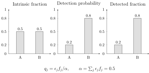
Selection alone can create an apparent population imbalance. Equal intrinsic fractions with detection probabilities 0.2 and 0.8 yield detected fractions 0.2 and 0.8. These are exact illustrative probabilities for two known classes without measurement error or contamination, not observational data.

Here inverse-efficiency counting works: $100/0.2=400/0.8=500$, recovering equal intrinsic counts. It fails for a class with zero efficiency, whose abundance is unconstrained by detections alone, and it is not a substitute for marginalizing uncertain event parameters in a real catalog.

The injection estimator

Suppose $N_{\mathrm{inj}}$ injections are drawn from proposal density $q(\theta,x)$ and passed through the search. Let $y_j=1$ if injection $j$ is recovered under the catalog rule and $0$ otherwise. Then

$$\widehat\alpha(\Lambda) = \frac{1}{N_{\mathrm{inj}}} \sum_{j=1}^{N_{\mathrm{inj}}} y_j \frac{\pi(\theta_j\mid\Lambda)p(x_j)}{q(\theta_j,x_j)}.$$

This estimator is valid only where the injection proposal has support wherever the target integrand is nonzero. A campaign concentrated on nearly equal-mass, nonspinning binaries cannot estimate selection for extreme mass ratios or precessing systems by reweighting alone.

Define recovered weights $w_j=y_j\pi(\theta_j\mid\Lambda)p(x_j)/q(\theta_j,x_j)$. A warning diagnostic is

$$N_{\mathrm{eff}} = \frac{\left(\sum_j w_j\right)^2}{\sum_j w_j^2}.$$

Large $N_{\mathrm{inj}}$ does not rescue a tiny $N_{\mathrm{eff}}$. For independent draws from the stated proposal, an unbiased estimate of the variance of the sample mean is

$$\widehat{\operatorname{Var}}(\widehat\alpha) =\frac{1}{N_{\mathrm{inj}}(N_{\mathrm{inj}}-1)} \sum_j(w_j-\widehat\alpha)^2.$$

Unrecovered injections still count: their $w_j=0$ values belong in the denominator and variance. Dividing by the number recovered instead of the number drawn would estimate the wrong quantity. Correlated or stratified injection designs require the corresponding variance calculation.

This accuracy matters increasingly as the catalog grows. A shape likelihood contains $-N\ln\alpha$, so a small numerical error gives $\delta\ln\mathcal L\simeq-N\,\delta\alpha/\alpha$. A selection estimate adequate for ten events may be inadequate for a thousand. Selection uncertainty must be propagated or shown negligible across the hyperparameter region being compared.

What the injections must reproduce

An injection campaign is faithful only if its recovery process matches the catalog construction in consequential respects:

Ingredient	Required match	Typical bias if omitted
Detector time	Duty cycle, sensitivity, PSD, glitches, data-quality masks	Wrong sensitive spacetime volume
Calibration	Epoch response and uncertainty treatment	Amplitude- and phase-dependent efficiency error
Waveform	Modes, spins, eccentricity, tides over target support	Missing or misranked source subpopulations
Search	Pipeline version, bank, ranking, coincidence, vetoes	Efficiency for the wrong decision rule
Threshold	Same FAR, rank, and de-duplication rule as catalog	Normalization inconsistent with included events
Injection proposal	Known density and full target support	Unstable or impossible reweighting

Software injections added to recorded strain test much of the analysis path but not the physical detector response before calibrated strain. Hardware injections test more of that chain but are sparse and are not a population Monte Carlo. The two serve different validation roles.

Selection in the catalog and population likelihoods

Conditioning on detection changes the distribution of observed sources:

$$p(\theta\mid\mathrm{det},\Lambda) = \frac{p_{\mathrm{det}}(\theta)\pi(\theta\mid\Lambda)}{\alpha(\Lambda)}.$$

For shape-only inference conditioned on $N$ detections, factors of $\alpha(\Lambda)^{-N}$ appear. In a Poisson rate model, the expected detected count contains the rate and selection exposure. Mixing these conventions can double-count or omit selection. The distinction and the correction to single-event conditioning are given in Thrane and Talbot 2019, § 5 and Appendices E–F, corrected PDF v9.

Selection generally does not become a per-event correction factor inserted into each already-detected event likelihood. It normalizes the detected ensemble under the same generative model. Applying “$1/p_{\mathrm{det}}$ weights” directly to noisy event estimates is not equivalent to the hierarchical likelihood and can be severely biased near threshold.

Convergence and failure diagnostics

A reproducible calculation records the injection table and proposal density, source/detector-frame conventions, waveform version, detector times, strain/calibration/data-quality release, pipeline and threshold version, random seed, and software environment. It then varies injection count and proposal design and reports $\widehat\alpha$, Monte Carlo uncertainty, and $N_{\mathrm{eff}}$ over the full hyperparameter domain.

Useful stress tests include:

• split by observing epoch, detector network, and pipeline;
• compare direct binomial estimates in well-populated cells with importance sampling;
• inject from a second proposal targeted at high-weight corners;
• perturb calibration, PSD, waveform family, and threshold;
• recover a mock population with known $\Lambda$; and
• deliberately choose an unsupported target to verify that the diagnostic fails loudly.

At the evidence cutoff 2026-08-18, an observational use must bind the official GWTC-5.0 release, the search and sensitivity specification in GWTC-5.0 Methods, §§ 2–3, and any release-specific selection products used by the population analysis LVK 2026, GWTC-5.0 Population, §§ 2–6 and appendices. This page reports no newly executed injection estimate and supplies no unverified rerun command.

Exercise

Sources are uniform in Euclidean volume within $0<D<D_{\max}$. A noiseless toy search detects every source with $D<D_h$ and none beyond, where $D_h<D_{\max}$.

1. Find the population selection fraction.
2. If injections are instead drawn uniformly in $D$, what importance factor, up to normalization, represents the volume population?

Solution

Uniform volume gives $\pi(D)=3D^2/D_{\max}^3$. Therefore

$$\alpha =\int_0^{D_h}\frac{3D^2}{D_{\max}^3}\,dD =\left(\frac{D_h}{D_{\max}}\right)^3.$$

For a proposal uniform in distance, $q(D)=1/D_{\max}$. The importance ratio is

$$\frac{\pi(D)}{q(D)} =\frac{3D^2}{D_{\max}^2},$$

so distant injections receive larger weights. If too few recovered injections lie near $D_h$, the weighted estimate can have low effective sample size even when the raw injection count is large.

References

• LIGO Scientific Collaboration, Virgo Collaboration, and KAGRA Collaboration (2026). “GWTC-5.0: Methods for Identifying and Characterizing Gravitational-Wave Transients.” arXiv:2605.27224. Open PDF.
• LIGO Scientific Collaboration, Virgo Collaboration, and KAGRA Collaboration (2026). “GWTC-5.0: Population Properties of Merging Compact Binaries.” arXiv:2605.27226. Open PDF.
• LIGO Scientific Collaboration, Virgo Collaboration, and KAGRA Collaboration (2026). GWTC-5.0 Data Release. DOI 10.7935/bk00-6a89. Official release.
• Thrane, E., and Talbot, C. (2019). “An Introduction to Bayesian Inference in Gravitational-Wave Astronomy: Parameter Estimation, Model Selection, and Hierarchical Models.” Publications of the Astronomical Society of Australia 36, e010. DOI. Open PDF v9, including the selection erratum.