Hyperboloidal Data and Conformal Infinity

A hyperboloidal hypersurface is spacelike but approaches null infinity rather than spatial infinity. It therefore combines an ordinary initial-value surface with direct access to the asymptotic radiation region. The central analytic difficulty is that conformal compactification turns infinity into a finite boundary while apparently introducing powers of the conformal factor in the equations. Smooth evolution requires both a regular conformal formulation and compatible asymptotic data.

Required background. Analysis for Mathematical Relativity supplies weighted regularity and elliptic estimates; The Einstein Equation supplies the constraints; Hypersurface Normals and Tangential Projectors supplies the geometry of the initial slice and its boundary.

Helpful background. Causality and Global Structure clarifies conformal boundaries, and PDEs and Green Functions for Gravitation supplies the evolution framework.

Hyperboloidal compactification

Let $(\mathcal M,g)$ be the physical spacetime. A conformal completion consists locally of a manifold with boundary $\widetilde{\mathcal M}$, a smooth nonnegative function $\Omega$, and an unphysical metric

$$\widetilde g=\Omega^2 g, \qquad \Omega=0, \qquad d\Omega\ne0 \quad\text{at }\mathscr I^+.$$

For asymptotically flat vacuum solutions, $\mathscr I^+$ is null with respect to $\widetilde g$. A hyperboloidal slice $\Sigma$ meets $\mathscr I^+$ transversely in a compact two-surface $\partial\Sigma$. Its physical metric $h$ is complete and noncompact, whereas $\widetilde h=\Omega^2h$ extends to the compact manifold with boundary $\overline\Sigma$.

This description fixes more than a rate of decay. The conformal factor has a rescaling freedom $\Omega\mapsto\vartheta\Omega$, $\widetilde g\mapsto\vartheta^2\widetilde g$. Statements about smoothness must therefore be conformally meaningful or made in a declared conformal gauge.

With the volume convention

$$K_{ij}=-h_i{}^\mu h_j{}^\nu\nabla_\mu n_\nu,$$

hyperboloidal vacuum data $(h,K)$ still obey the Hamiltonian and momentum constraints. Their compactified form is a singular elliptic system unless the leading boundary terms cancel.

Boundary regularity and the shear-free condition

The conformal transformation of curvature contains terms proportional to $\Omega^{-1}$ and $\Omega^{-2}$. Regular conformal field equations promote suitable rescaled curvature variables to independent unknowns and use the constraints to cancel these apparent singularities. This succeeds only when the data have compatible asymptotic expansions.

At the first nontrivial order, the outgoing null congruence generated from $\partial\Sigma$ must be shear-free at $\mathscr I^+$. Geometrically, a trace-free combination of the second fundamental form of $\partial\Sigma$ in $(\overline\Sigma,\widetilde h)$ and the rescaled trace-free part of $K$ must vanish. The invariant statement is safer than a formula copied between conformal gauges: both ingredients change under rescaling, while their compatibility expresses regularity of the outgoing null geometry.

If this condition or higher compatibility conditions fail, solving the constraints may produce terms such as $\Omega^k\log\Omega$. Such polyhomogeneous data can still define meaningful asymptotics, but they do not yield a smooth conformal boundary of the claimed differentiability. Andersson explains the regularity problem and the shear-free boundary condition in Andersson 2002, §§1–4.

A conformal local-existence statement

A representative theorem has the following form. Let smooth vacuum hyperboloidal data be given on a compact three-manifold with boundary. Assume the physical constraints hold in the interior, the conformally rescaled fields extend smoothly to the boundary, the boundary is the intended cut of null infinity, and the complete hierarchy of compatibility conditions required by the chosen conformal formulation is satisfied. Then the regular conformal Einstein equations have a unique smooth solution for a finite conformal time. On the region $\Omega>0$, the metric $g=\Omega^{-2}\widetilde g$ solves the physical vacuum equations, and $\Omega=0$ supplies a smooth local portion of $\mathscr I^+$.

The proof architecture is:

1. solve the conformal constraint equations on $\overline\Sigma$;
2. choose a conformal and coordinate gauge in which the enlarged conformal system is symmetric hyperbolic;
3. apply local energy estimates on the compact domain;
4. propagate the conformal constraints and the condition defining $\Omega$;
5. restrict to $\Omega>0$ to recover the physical development.

This is a theorem about data satisfying a strong boundary regularity package. It does not say that every asymptotically flat Cauchy data set admits a smooth $\mathscr I^+$, nor that local conformal existence implies future completeness. The rescaled curvature data are part of the hypotheses: smoothness of $\widetilde h$ alone is not enough. Friedrich and Rendall separate local evolution from global conclusions in Friedrich and Rendall 2000, §6.

Hyperboloidal slicing versus compactification

Changing the time slices and rescaling the metric solve different problems. A hyperboloidal time function makes slices approach null infinity. A conformal factor makes that infinity a finite coordinate location. One may use hyperboloidal slices without evolving conformal field equations, in which case formally singular coefficients must be regularized or handled analytically. Zenginoğlu develops this distinction and the regularity conditions for hyperboloidal evolution in Zenginoğlu 2008, §§2–4, equations (1)–(18).

Nor is $\mathscr I^+$ a timelike outer boundary. Its characteristic nature means no arbitrary incoming physical data may be prescribed there. Timelike boundaries, treated on the Einstein initial-boundary page, require a different boundary-flux analysis.

A Minkowski hyperboloid and its conformal diagram

In Minkowski spacetime take $t=\sqrt{r^2+a^2}$ with $a\gt0$. Since $dt/dr=r/\sqrt{r^2+a^2}\lt1$, the slice is spacelike even though its slope approaches that of a radial null ray. Its induced metric is

$$h=\frac{a^2}{r^2+a^2}\,dr^2+r^2d\omega^2,$$

and, with the convention above and the future normal, $K_{ij}=-a^{-1}h_{ij}$. Put $x=1/r$ and choose $\Omega=x$. Since $dr=-x^{-2}dx$,

$$\widetilde h=\Omega^2h =\frac{a^2}{1+a^2x^2}\,dx^2+d\omega^2.$$

The compactified metric extends smoothly to $x=0$, where the boundary is a round sphere. The coordinate $x=1/r$ is used only near infinity; another regular chart covers the center. Its boundary has vanishing trace-free second fundamental form, and $K$ has no trace-free part, so the shear-free condition is satisfied.

To see which infinity is reached, compactify the full radial spacetime. Use dimensionless null angles

$$\begin{gathered} U=\arctan\frac{t-r}{a},\qquad V=\arctan\frac{t+r}{a},\\ T=U+V,\qquad R=V-U,\qquad \Omega_{\mathrm P}=2\cos U\cos V=\cos T+\cos R. \end{gathered}$$

Then

$$\Omega_{\mathrm P}^2g =a^2\left(-dT^2+dR^2+\sin^2R\,d\omega^2\right).$$

The physical domain is $R\ge0$, $|T|+R\lt\pi$. Radial null rays have slope $\pm1$, so conformal compactification preserves the light cones. On the hyperboloid, $(t-r)(t+r)=a^2$ and both factors are positive; hence $T=\pi/2$. It ends at $(T,R)=(\pi/2,\pi/2)$ on $\mathscr I^+$. The plane $t=0$ instead has $T=0$ and ends at $(0,\pi)$, spatial infinity $i^0$.

The figure displays these exact transformed slices. Inspect the different endpoints: a hyperboloidal slice intersects a regular spherical cut of null infinity, while an asymptotically Euclidean slice approaches spatial infinity.

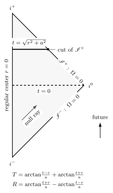
Minkowski spacetime in the spherical radial quotient, using the exact $(T,R)$ transformation above with the same scale on both axes. The solid hyperboloid is $T=\pi/2$; the dashed Cauchy slice is $T=0$. Each interior diagram point represents a symmetry two-sphere, and the marked cut of $\mathscr I^+$ is a sphere. Conformal coordinates preserve causal directions but not physical distances.

A hyperboloid is not a Cauchy surface for all of Minkowski spacetime. For example, a future-inextendible causal curve whose retarded time $u=t-r$ stays negative never reaches this $u\gt0$ slice. Hyperboloidal evolution concerns its own domain of dependence and the associated portion of null infinity.

Check your understanding

For the conformal factor $\Omega_{\mathrm P}=\cos T+\cos R$, verify that its gradient is nonzero and null at the marked cut. Why does the same regular-boundary argument not apply at $i^0$?

Solution

At $T=R=\pi/2$, $d\Omega_{\mathrm P}=-dT-dR$. The radial inverse conformal metric gives $|d\Omega_{\mathrm P}|^2=a^{-2}(-1+1)=0$, while the covector itself is nonzero. Thus this is a regular null boundary. At $i^0$, $(T,R)=(0,\pi)$, both derivatives vanish. Spatial infinity is an exceptional endpoint of this compactification, not another regular point of the null hypersurface. These checks establish the geometry of the explicit flat example; they do not prove smooth conformal infinity for perturbed data.

References

• Andersson, Lars. “Construction of Hyperboloidal Initial Data.” arXiv:gr-qc/0205083, 2002.
• Friedrich, Helmut, and Alan D. Rendall. “The Cauchy Problem for the Einstein Equations.” In Einstein’s Field Equations and Their Physical Implications, Lecture Notes in Physics 540, 127–224. Springer, 2000. arXiv:gr-qc/0002074.
• Zenginoğlu, Anıl. “Hyperboloidal Evolution with the Einstein Equations.” Classical and Quantum Gravity 25 (2008): 195025. arXiv:0808.0810.