Statistical Ensembles and Partition Functions

An ensemble specifies both what a system can exchange and how its microscopic states are weighted. The logarithm of its partition function is a generating function: first derivatives give mean conserved quantities, second derivatives give fluctuations, and a Legendre transform gives the appropriate thermodynamic potential. Different ensembles model different physical couplings, not merely different calculation tricks.

Required background. Calculus and Linear Algebra supplies constrained extrema, second derivatives, and eigenvalue language. The probability weights and Gaussian saddle used below are defined locally. Helpful background. Classical and Variational Mechanics supplies phase-space and conservation-law language; Quantum Mechanics supplies energy-state and spectral language, while the Bose and Fermi occupation rules in the optional bridge below are introduced locally.

Three equilibrium ensembles

For an isolated system with energy in a narrow shell around $E$, volume $V$, and particle number $N$, let $\mathcal N_E(E,V,N)$ be the number of accessible states in that shell. The microcanonical assignment is uniform:

$$p_i=\frac{1}{\mathcal N_E}, \qquad S(E,V,N)=\ln\mathcal N_E.$$

The shell convention matters for finite systems, but its microscopic width does not affect the leading extensive entropy when it is broad compared with the level spacing and narrow on macroscopic scales. Ergodicity can help explain why long-time measurements explore this distribution in some systems; it is not part of the ensemble’s algebraic definition.

If the system is weakly coupled to a much larger reservoir, so the interaction energy is negligible in the equilibrium accounting, a system microstate of energy $E_i$ leaves the bath with energy $E_{\mathrm{tot}}-E_i$. Expanding the bath entropy gives

$$S_R(E_{\mathrm{tot}}-E_i) =S_R(E_{\mathrm{tot}})-\beta E_i -\frac{E_i^2}{2T^2C_R}+\cdots.$$

When the reservoir heat capacity $C_R$ is large enough that the quadratic correction is negligible over the system’s relevant energies, the number of compatible bath states is proportional to $e^{-\beta E_i}$. Normalization then gives the canonical weights

$$p_i=\frac{e^{-\beta E_i}}{Z(\beta,V,N)}, \qquad Z=\sum_i e^{-\beta E_i}, \qquad \beta=\frac{1}{T}.$$

We use $k_{\mathrm B}=1$, natural logarithms, and $T\gt 0$ unless a bounded-spectrum exception is explicitly stated. At fixed $(V,N)$, differentiating $Z$ yields

$$U=\langle E\rangle=-\frac{\partial\ln Z}{\partial\beta}, \qquad \operatorname{Var}(E)=\frac{\partial^2\ln Z}{\partial\beta^2},$$

and substitution into $S=-\sum_i p_i\ln p_i$ gives

$$S=\ln Z+\beta U, \qquad F=U-TS=-T\ln Z.$$

The first derivative is the mean energy and the second is a nonnegative variance, so $\ln Z$ is convex in $\beta$. The reservoir construction and these identities are derived in Tong, current notes, §1.3, printed pp. 17–25.

The canonical law can also be characterized variationally. Maximize Gibbs entropy at fixed normalization and mean energy:

$$\mathcal L[p] =-\sum_i p_i\ln p_i -\alpha\left(\sum_i p_i-1\right) -\beta\left(\sum_i p_iE_i-U\right).$$

Stationarity with respect to every positive $p_i$ gives $\ln p_i=-1-\alpha-\beta E_i$; normalization then identifies $e^{1+\alpha}=Z$. Because $-\sum_i p_i\ln p_i$ is strictly concave on a finite probability simplex, this stationary distribution is the unique maximum whenever the prescribed mean energy lies strictly between the lowest and highest levels. At an endpoint, the maximum is instead the uniform distribution on the corresponding extremal-energy eigenspace, obtained as a limiting Gibbs state. For a nonconstant finite spectrum, a mean energy above the uniform distribution’s mean requires $\beta\lt0$; that bounded-spectrum case is outside the positive-temperature branch used here. The variational argument does not say that every isolated trajectory becomes canonical: it identifies a probability law after a mean-energy constraint and state space have been chosen.

When energy and particles are exchanged, the reservoir expansion contains $-\beta(E_i-\mu N_i)$. In the quantum description this simple joint weighting assumes $[H,N]=0$. The grand-canonical ensemble is

$$p_i=\frac{e^{-\beta(E_i-\mu N_i)}}{\Xi}, \qquad \Xi=\sum_i e^{-\beta(E_i-\mu N_i)}, \qquad \Omega=-T\ln\Xi.$$

Here $\Xi$ is the grand partition function and $\Omega$ is the grand potential, not the microcanonical count. At fixed $(T,V)$,

$$\langle N\rangle=T\left(\frac{\partial\ln\Xi}{\partial\mu}\right)_{T,V}, \qquad \operatorname{Var}(N) =T\left(\frac{\partial\langle N\rangle}{\partial\mu}\right)_{T,V} =T^2\left(\frac{\partial^2\ln\Xi}{\partial\mu^2}\right)_{T,V}.$$

Volume differentiation supplies the equation of state,

$$p=T\left(\frac{\partial\ln\Xi}{\partial V}\right)_{T,\mu}.$$

For a homogeneous extensive phase in the thermodynamic limit, Euler scaling then gives $\Omega=-pV$. Boundaries and other subextensive corrections prevent that last equality from being exact for a generic finite system.

The three main ensembles can therefore be read as a control-and-weight table:

Ensemble	Quantities held fixed	Microscopic weight	Generated potential
Microcanonical	$E,V,N$	uniform in an energy shell	$S=\ln\mathcal N_E$
Canonical	$T,V,N$	$e^{-\beta E_i}/Z$	$F=-T\ln Z$
Grand canonical	$T,V,\mu$	$e^{-\beta(E_i-\mu N_i)}/\Xi$	$\Omega=-T\ln\Xi$

Optional bridge: Bose and Fermi occupation laws

For noninteracting identical quantum particles, it is convenient to sum over the occupation number $n_r$ of each one-particle mode with energy $\epsilon_r$. Let $q_r=e^{-\beta(\epsilon_r-\mu)}$. A bosonic mode permits $n_r=0,1,2,\ldots$, so

$$\Xi_r^{\mathrm B}=\sum_{n=0}^{\infty}q_r^n=\frac{1}{1-q_r}, \qquad \langle n_r\rangle_{\mathrm B} =\frac{1}{e^{\beta(\epsilon_r-\mu)}-1}.$$

Convergence requires $\mu\lt \epsilon_r$ for every mode, hence $\mu$ cannot exceed the lowest one-particle energy. A fermionic mode permits only $n_r=0,1$, so

$$\Xi_r^{\mathrm F}=1+q_r, \qquad \langle n_r\rangle_{\mathrm F} =\frac{1}{e^{\beta(\epsilon_r-\mu)}+1}.$$

When $e^{\beta(\epsilon_r-\mu)}\gg1$, both reduce to the dilute Maxwell–Boltzmann occupation $e^{-\beta(\epsilon_r-\mu)}$. These formulas assume noninteracting modes and equilibrium; interactions can invalidate the factorization even though the grand-canonical definition remains meaningful. Tong derives the Bose–Einstein and Fermi–Dirac laws in Tong, current notes, §§3.5.1 and 3.6, printed pp. 78–81 and 90–92.

When ensembles agree

The saddle-point bridge makes the canonical–microcanonical relation explicit. Let $g(E)\,dE$ count states and choose one fixed reference width $\Delta E_0$. Define

$$S_\Delta(E)=\ln\!\left[g(E)\Delta E_0\right].$$

Then both the logarithm and the canonical measure are dimensionless:

$$Z(\beta) =\int\frac{dE}{\Delta E_0} e^{S_\Delta(E)-\beta E}.$$

Changing the fixed reference width adds a constant to $S_\Delta$ and does not change the saddle. Each finite canonical system fixes $(V,N)$. Suppose a no-exchange thermodynamic sequence has $V,N\to\infty$ at fixed specific volume $v=V/N$, one interior dominant energy $E_*$, and a twice-differentiable, strictly concave entropy near that point. Then

$$S'(E_*)=\beta=\frac{1}{T}, \qquad S''(E_*)=-\frac{1}{T^2C_V}.$$

Thus $C_V\gt 0$ makes the stationary point a local maximum. Expanding the exponent to second order gives a Gaussian with $\operatorname{Var}(E)=T^2C_V$. When $C_V$ grows proportionally to $N$ at fixed temperature, the standard deviation of the energy per particle is $\sqrt{\operatorname{Var}(E)}/N=O(N^{-1/2})$. The relative width $\sqrt{\operatorname{Var}(E)}/|E_*|$ has the same scaling if the limiting mean energy per particle is nonzero; unlike that ratio, the fluctuation of energy per particle is unaffected by shifting the energy zero. This scaling can fail at critical points, and at first-order coexistence two competing saddles can produce a bimodal distribution rather than one Gaussian. A negative microcanonical heat-capacity branch has $S''\gt 0$ and cannot be an ordinary canonical maximum.

For ordinary additive systems with short-range interactions and a well-defined thermodynamic limit, strict concavity in energy and a unique smooth saddle usually produce canonical–microcanonical concentration after matching $E$ and $T$. For this no-exchange limit, write

$$s(e,v)=\lim_{N\to\infty}\frac{S_N(Ne,Nv,N)}{N}, \qquad e=\frac{E}{N},\quad v=\frac{V}{N}.$$

Extending the conclusion to particle exchange instead uses the entropy per volume $s_V(e_V,n)=\lim_{V\to\infty}S_V(e_VV,V,nV)/V$, with $e_V=E/V$ and $n=N/V$. It requires concentration in both densities and the corresponding joint concavity or large-deviation hypotheses; energy concavity alone is insufficient. Tong demonstrates the regular single-energy-saddle concentration in Tong, current notes, §1.3.2, printed pp. 19–21.

The sharper fixed-$v$ geometry suppresses the constant specific volume and writes $s(e)=s(e,v)$. A canonical inverse temperature $\beta$ realizes a microcanonical energy $e$ when $s$ has a supporting line there:

$$s(e')\leq s(e)+\beta(e'-e) \quad\text{for every allowed }e'.$$

The figure turns that inequality into geometry. In the upper panel, inspect how the positive-slope tangent at $e_\star$ stays above the entire entropy curve. In the lower panel, compare the depressed point $e_0$ with the positive-slope common tangent through the two outer contact points: no line through $(e_0,s(e_0))$ can lie above both sides.

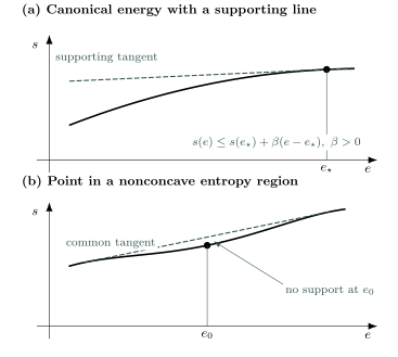
A microcanonical energy is canonically realizable only where $s(e)$ admits a supporting line. Panel (a) shows a strict positive-$\beta$ supporting tangent at $e_\star$, while panel (b) places $e_0$ in a nonconcave region of $s$ below a positive-slope common tangent, so no $\beta$ supports it and no canonical ensemble selects it as equilibrium. Original schematic; axes not to scale.

Any supporting line gives thermodynamic equivalence at that energy. Under the corresponding large-deviation hypotheses, strict support gives equality of the canonical and microcanonical equilibrium-macrostate sets, while nonstrict support generally gives only inclusion and permits several energies at one $\beta$. Vanishing specific relative entropy can still hold in the nonstrict case; equality at the stronger specific-action level needs an additional concentration condition. At a point where $s$ has no supporting line, that energy is absent from every canonical equilibrium-energy set. Touchette separates these levels in Touchette 2015, Proposition 2, author-manuscript pp. 11–12; Theorem 7, p. 16; and Theorems 10 and 12, pp. 20–22 (Open PDF), and treats the additional particle-density saddle for canonical–grand-canonical equivalence in §VI.A, pp. 24–25.

Finite systems have nonzero fluctuations and surface corrections. Long-range nonadditive interactions make subsystem–reservoir separation delicate. Self-gravitating matter is the central warning for this site: the canonical variance identity forbids $C_V\lt 0$, while an isolated gravitating system may possess a negative microcanonical caloric slope. One must state the ensemble before calling either result unstable.

Agreement of thermodynamic potentials need not imply equality of finite-size probability distributions, and agreement of equilibrium macrostates need not make rare-event probabilities identical. Conversely, a local observable can agree between ensembles even when a global fluctuation does not. A static ensemble comparison specifies the observable, the matched intensive parameters, and the thermodynamic limit; convergence of long-time averages is a separate dynamical question.

Exercise: a two-level system

For $N$ independent distinguishable units with energies $0$ and $\epsilon\gt0$, find the canonical internal energy and heat capacity, and check their low- and high-temperature limits.

Solution

The one-unit and total partition functions are

$$Z_1=1+e^{-\beta\epsilon}, \qquad Z=Z_1^N.$$

Therefore

$$U=-\partial_\beta\ln Z =\frac{N\epsilon}{e^{\beta\epsilon}+1},$$

and

$$C_V=\frac{\partial U}{\partial T} =N(\beta\epsilon)^2 \frac{e^{\beta\epsilon}}{(1+e^{\beta\epsilon})^2}\geq0.$$

At low temperature the excited state freezes out, so $U,C_V\to0$. At high temperature both levels are equally populated, $U\to N\epsilon/2$, while the finite spectrum again makes $C_V\to0$. The heat capacity therefore has a Schottky peak at an intermediate temperature. The partition function produces both limits and the stability sign without tracking individual configurations.

The next page, Entropy, Relative Entropy, and Information, separates the physical meanings attached to the logarithms used here.

References

• Tong, David. Statistical Physics. University of Cambridge Part II Mathematical Tripos lecture notes, current official undated-cover PDF, §§1.2–1.4, printed pp. 2–30; §§3.5.1 and 3.6, printed pp. 78–81 and 90–92. Open PDF.
• Touchette, Hugo. “Equivalence and Nonequivalence of Ensembles: Thermodynamic, Macrostate, and Measure Levels.” Journal of Statistical Physics 159 (2015): 987–1016, §§III–VI.A. doi:10.1007/s10955-015-1212-2; Open PDF.