Advanced, Retarded, and Causal Propagators

Advanced and retarded Green operators solve the same sourced wave equation but impose opposite causal support. Their difference cancels the source and produces a homogeneous, spacelike-compact solution. More strongly, every such solution is obtained this way, and two compact sources produce the same solution exactly when they differ by the field equation applied to another compact test section.

For the local PDE bridge, a compact test section $f$ represents a localized source and a distributional identity $PGf=f$ means equality after pairing with every compact smooth dual test section. Support records where those pairings can be nonzero. A causal Green operator is therefore both an inverse on tests and a rule selecting a causal support class.

Required background. Partial Differential Equations and Green Functions provides distributional kernels, inverse identities, and causal support; Classical Field Theory supplies linear field equations and their compactly supported source interpretation. Helpful background. Flat-Spacetime Quantum Field Theory provides propagators and mode solutions; Causality and Global Structure establishes causal futures, causal pasts, Cauchy surfaces, and global hyperbolicity.

Green operators and causal support

Assume $E\to M$ is a smooth finite-rank vector bundle, $P:C^\infty(M,E)\to C^\infty(M,E)$ is normally hyperbolic with smooth coefficients, and $M$ is a smooth globally hyperbolic spacetime without timelike boundary. We use names rather than superscripts because sign and advanced/retarded labels vary across sources. Define

$$\begin{aligned} &PG_{\mathrm{ret}}f=f, &&G_{\mathrm{ret}}Pf=f, &&\operatorname{supp}(G_{\mathrm{ret}}f) \subset J^+(\operatorname{supp}f),\\ &PG_{\mathrm{adv}}f=f, &&G_{\mathrm{adv}}Pf=f, &&\operatorname{supp}(G_{\mathrm{adv}}f) \subset J^-(\operatorname{supp}f), \end{aligned}$$

for every $f\in C_c^\infty(M,E)$. Thus the retarded solution vanishes before the source can influence it, while the advanced solution vanishes after the source’s influence has been propagated backward. Existence and uniqueness follow from the global Cauchy theorem by imposing zero data on a Cauchy surface entirely to the past or future of the compact source. The full construction and inverse identities are proved in Bär, Ginoux, and Pfäffle 2007, §3.4, pp. 88–92.

The figure shows the support bound, not a ray-by-ray solution. Its compact source is drawn as a diamond $K$ in a flat one-space, one-time schematic. The dashed lines are the null boundaries of $J^\pm(K)$; both causal sets include the source diamond. Shaded interiors indicate where propagation is permitted, not where a particular solution must be nonzero. In curved spacetime or for massive fields, tails can fill regions inside the null boundary.

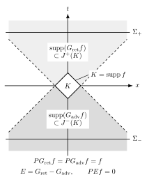
A compact source $K$ has retarded support within $J^+(K)$ and advanced support within $J^-(K)$. Their source terms cancel, so $E f$ is homogeneous everywhere. The flat two-dimensional causal geometry is schematic; shading indicates allowed support, not field amplitude or a claim of nonzero tails.

Semantically, there are three relationships to retain: $G_{\mathrm{ret}}f$ occupies only $J^+(\operatorname{supp}f)$, $G_{\mathrm{adv}}f$ occupies only $J^-(\operatorname{supp}f)$, and both solve $Pu=f$. The two displayed Cauchy surfaces emphasize that either solution can be selected by zero data on the appropriate side of the source.

The causal propagator removes the source

Fix the sign

$$E\equiv G_{\mathrm{ret}}-G_{\mathrm{adv}}.$$

Both inverse identities immediately give

$$PEf=0, \qquad EPf=0.$$

The first equation says that $Ef$ is a homogeneous solution even though each term separately solves the sourced equation. The support inclusion

$$\operatorname{supp}(Ef) \subset J(\operatorname{supp}f)$$

makes it spacelike compact: its intersection with every Cauchy hypersurface is compact. The second equation says that changing the source by $Ph$, with $h$ compactly supported, does not change the solution. Hence $E$ descends to a map

$$\overline E: C_c^\infty(M,E)/P C_c^\infty(M,E) \longrightarrow \operatorname{Sol}_{\mathrm{sc}}(P).$$

The point is not merely that the map is defined. It is an isomorphism.

Exactness of the source-to-solution sequence

The source-to-solution statement is the exact sequence below, with exactness asserted at each term having an incoming and an outgoing arrow:

$$0\longrightarrow C_c^\infty(M,E) \xrightarrow{\ P\ } C_c^\infty(M,E) \xrightarrow{\ E\ } C_{\mathrm{sc}}^\infty(M,E) \xrightarrow{\ P\ } C_{\mathrm{sc}}^\infty(M,E).$$

Exactness at each position has a concrete meaning.

First, $P$ is injective on compactly supported sections: if $Ph=0$, then $h=G_{\mathrm{ret}}Ph=0$. Second, if $Ef=0$, the two Green solutions agree. Set

$$h=G_{\mathrm{ret}}f=G_{\mathrm{adv}}f.$$

Its support lies in the intersection $J^+(\operatorname{supp}f)\cap J^-(\operatorname{supp}f)$, which is compact by global hyperbolicity, and $Ph=f$. Therefore $\ker E=\operatorname{im}P$ on compact tests.

Third, take any spacelike-compact homogeneous solution $u$. Split it with a smooth partition into a past-supported part $u_-$ and a future-supported part $u_+$ across a finite Cauchy slab. Because $Pu=0$, the section

$$f=Pu_+=-Pu_-$$

is supported only where the cutoff changes and is therefore compact. Applying the inverse and support properties shows $G_{\mathrm{ret}}f=u_+$ and $G_{\mathrm{adv}}f=-u_-$, so $Ef=u$. This proves $\ker P=\operatorname{im}E$ on spacelike-compact sections. The proof, including the support intersections that justify integration by parts, is Bär, Ginoux, and Pfäffle 2007, Theorem 3.4.7, pp. 90–91.

Formal self-adjointness was not used to establish this exact sequence. It becomes consequential when a fiber pairing is used to turn $E$ into an antisymmetric bilinear form. For a formally self-adjoint scalar operator,

$$\int_M f\,Eh\,dV_g =-\int_M h\,Ef\,dV_g,$$

and the declared sign of $E$ fixes the sign of the symplectic form and, after quantization, the commutator. The algebraic source-to-solution correspondence is summarized in Hollands and Wald 2015, §2.1, Eqs. (5)–(10).

Flat-spacetime sign check

For the massless scalar in four-dimensional Minkowski spacetime with our operator $\Box=-\partial_t^2+\nabla^2$, distributional kernels satisfying $\Box G=\delta^{(4)}$ are

$$G_{\mathrm{ret}}(t,\mathbf x) =-\frac{\delta(t-r)}{4\pi r}, \qquad G_{\mathrm{adv}}(t,\mathbf x) =-\frac{\delta(t+r)}{4\pi r}, \qquad r=\lvert\mathbf x\rvert.$$

The first is supported on the future null cone and the second on the past null cone. Therefore

$$E(t,\mathbf x) =-\frac{\delta(t-r)-\delta(t+r)}{4\pi r},$$

which is odd under $t\mapsto -t$ and solves the homogeneous equation distributionally everywhere: the two delta-function sources at the origin cancel. The overall minus sign is forced by the wave operator; using the opposite metric signature without translating the kernel would reverse it. A useful independent normalization check is $E(0,\mathbf x)=0$ and $\partial_tE(0,\mathbf x)=-\delta^{(3)}(\mathbf x)$. It makes $[\Phi(t,\mathbf x),\partial_t\Phi(t,\mathbf y)]=i\delta^{(3)}(\mathbf x-\mathbf y)$ when $[\Phi(x),\Phi(y)]=iE(x,y)$. Massive fields and generic curved geometries develop interior tails, but the causal support inclusions remain unchanged.

Limitations and the role of global hyperbolicity

Normal hyperbolicity is local, whereas uniqueness of both Green operators is global. A timelike boundary can admit several reflecting, transmitting, or dissipative choices, each producing a different Green operator. On a compact Lorentzian spacetime, even existence of a two-sided Green inverse can fail because constants lie in the kernel of $\Box$. The exact sequence above therefore does not extend unchanged to arbitrary causal domains.

The next page uses the quotient isomorphism and the conserved current to build covariant phase space. That construction remains sensitive to the sign of $E$ but not to which compact representative $f$ is chosen.

Check your understanding

Let $f'=f+Ph$ with $f,h\in C_c^\infty(M,E)$. Show that $f$ and $f'$ define the same spacelike-compact solution, and identify exactly which Green-operator identity is used.

Solution

Compute $Ef'=Ef+EPh$. Because both Green operators are left inverses of $P$ on compact test sections, $G_{\mathrm{ret}}Ph=h=G_{\mathrm{adv}}Ph$. Their difference therefore gives $EPh=0$, so $Ef'=Ef$. This check explains why the natural source space is the quotient by $P C_c^\infty$. It also separates the two inverse identities: $EP=0$ establishes independence of the representative, whereas $PE=0$ establishes that the resulting field is a homogeneous solution. Both are needed for the source-to-solution isomorphism.

References

• Bär, Christian, Nicolas Ginoux, and Frank Pfäffle. Wave Equations on Lorentzian Manifolds and Quantization. ESI Lectures in Mathematics and Physics. Zürich: European Mathematical Society, 2007. DOI 10.4171/037.
• Hollands, Stefan, and Robert M. Wald. “Quantum Fields in Curved Spacetime.” Physics Reports 574 (2015): 1–35. DOI 10.1016/j.physrep.2015.02.001.