Cosmological Particle Creation

Cosmological particle creation is positive–negative frequency mixing between two physically selected mode bases. It is unambiguous when the expansion history has suitable stationary or adiabatic in and out regimes; at an intermediate time, an “occupation number” depends on the chosen instantaneous basis. The production amplitude is controlled by the failure of the mode frequency to vary adiabatically, including turning points that defeat a simple WKB expansion.

Required background. Compactly, a normalized pair of oscillator solutions forms a symplectic basis, and Cauchy evolution preserves their Wronskian; distributional mode sums define the state only after their ultraviolet behavior is controlled. Partial Differential Equations and Green Functions supplies that evolution and distribution framework. Helpful background. Flat-Spacetime Quantum Field Theory provides creation operators and oscillator vacua; Causality and Global Structure establishes the initial and final Cauchy regions; Quantum Fields in Curved Spacetime provides Bogoliubov states and renormalized observables.

In and out particle bases

Let a rescaled scalar mode satisfy

$$\chi_k''+\omega_k^2(\eta)\chi_k=0, \qquad \chi_k\chi_k^{*\prime}-\chi_k^*\chi_k'=i.$$

Assume $\omega_k$ tends to positive constants $\omega_{k,\mathrm{in}}$ and $\omega_{k,\mathrm{out}}$ as $\eta\to-\infty$ and $+\infty$. These asymptotic time-translation symmetries select normalized solutions

$$u_{k,\mathrm{in}}\sim\frac{e^{-i\omega_{k,\mathrm{in}}\eta}} {\sqrt{2\omega_{k,\mathrm{in}}}}, \qquad u_{k,\mathrm{out}}\sim\frac{e^{-i\omega_{k,\mathrm{out}}\eta}} {\sqrt{2\omega_{k,\mathrm{out}}}}.$$

Since each pair $\{u_k,u_k^*\}$ spans the solution space,

$$u_{k,\mathrm{in}} =\alpha_k u_{k,\mathrm{out}} +\beta_k u_{k,\mathrm{out}}^*, \qquad |\alpha_k|^2-|\beta_k|^2=1.$$

The Wronskian gives the last identity. If the state is the in-vacuum, the mean number of out-quanta is

$$\langle0_{\mathrm{in}}| N_{\mathbf k,\mathrm{out}} |0_{\mathrm{in}}\rangle=|\beta_k|^2.$$

For a continuum, the physical number density in the late-time region is

$$n_{\mathrm{out}}(t) =\frac{1}{a^3(t)} \int\frac{d^3k}{(2\pi)^3}|\beta_k|^2.$$

The factor $a^{-3}$ converts a comoving count to a physical density. Finiteness also requires sufficient ultraviolet falloff; modewise finite $|\beta_k|$ does not alone guarantee a finite total number.

Differential equations for mixing

To see what drives $\beta_k$, define

$$\Theta_k(\eta)=\int^\eta\omega_k(\eta')\,d\eta'$$

and decompose an exact solution as

$$\chi_k=\frac{1}{\sqrt{2\omega_k}} \left(\alpha_k e^{-i\Theta_k}+\beta_k e^{i\Theta_k}\right),$$

with the auxiliary condition

$$\chi_k'=-i\sqrt{\frac{\omega_k}{2}} \left(\alpha_k e^{-i\Theta_k}-\beta_k e^{i\Theta_k}\right).$$

Substitution into the oscillator equation yields

$$\alpha_k'=\frac{\omega_k'}{2\omega_k} e^{2i\Theta_k}\beta_k, \qquad \beta_k'=\frac{\omega_k'}{2\omega_k} e^{-2i\Theta_k}\alpha_k.$$

These equations preserve $|\alpha_k|^2-|\beta_k|^2$. Starting with $\alpha_k=1$, $\beta_k=0$, the leading result is

$$\beta_k(+\infty)\simeq \int_{-\infty}^{+\infty}d\eta\, \frac{\omega_k'}{2\omega_k} \exp[-2i\Theta_k(\eta)].$$

Rapid phase oscillations suppress the integral when

$$\epsilon_{1,k}=\left|\frac{\omega_k'}{\omega_k^2}\right|\ll1$$

and the corresponding higher-derivative ratios are small. This is a useful criterion, not a universal one-number law: near a real zero of $\omega_k^2$, or a nearby complex turning point, the WKB basis changes character and Stokes matching controls production. Parker’s original expanding-universe calculation establishes the mode-mixing mechanism in Parker 1969, complete article, pp. 1057–1068.

A solvable smooth frequency quench

Consider the positive frequency profile

$$\omega_k^2(\eta) =\frac{\omega_{k,\mathrm{in}}^2+\omega_{k,\mathrm{out}}^2}{2} +\frac{\omega_{k,\mathrm{out}}^2-\omega_{k,\mathrm{in}}^2}{2} \tanh\left(\frac{\eta}{\tau}\right).$$

Here $\tau\gt0$ is a conformal-time transition scale and both asymptotic frequencies are positive. This oscillator is realized by a massive, conformally coupled scalar in four dimensions if $a^2(\eta)$ interpolates by the same tanh profile between positive constants $a_{\rm in}^2$ and $a_{\rm out}^2$: then $\omega_{k,j}^2=k^2+m^2a_j^2$. An arbitrary minimally coupled scalar does not have this simple profile, because its frequency also contains $-a''/a$.

The connection calculation can be followed explicitly. Suppress $k$ and set $\omega_\pm=(\omega_{\rm out}\pm\omega_{\rm in})/2$ and $z=[1+\tanh(\eta/\tau)]/2$. An in-mode is

$$\begin{aligned} u_{\rm in}(\eta)&=\frac{e^{-i\omega_+\eta} [2\cosh(\eta/\tau)]^{-i\tau\omega_-}} {\sqrt{2\omega_{\rm in}}}\\ &\quad\times{}_2F_1\left(1+i\tau\omega_-,i\tau\omega_-; 1-i\tau\omega_{\rm in};z\right). \end{aligned}$$

At $\eta\to-\infty$, $z\to0$ and the prefactor tends to $e^{-i\omega_{\rm in}\eta}/\sqrt{2\omega_{\rm in}}$. Continuing the hypergeometric function to $z\to1$ gives the negative-frequency coefficient

$$\beta=\sqrt{\frac{\omega_{\rm out}}{\omega_{\rm in}}} \frac{\Gamma(1-i\tau\omega_{\rm in})\Gamma(i\tau\omega_{\rm out})} {\Gamma(i\tau\omega_-)\Gamma(1+i\tau\omega_-)}.$$

The continuation formula and $|\Gamma(iy)|^2=\pi/[y\sinh(\pi y)]$ are given in NIST DLMF, n.d., Eq. 15.8.4 and NIST DLMF, n.d., Eq. 5.4.3. Together with $\Gamma(1+iy)=iy\Gamma(iy)$, they give

$$|\beta_k|^2 =\frac{ \sinh^2\!\left[\frac{\pi\tau}{2} (\omega_{k,\mathrm{out}}-\omega_{k,\mathrm{in}})\right]} {\sinh(\pi\tau\omega_{k,\mathrm{in}}) \sinh(\pi\tau\omega_{k,\mathrm{out}})}.$$

The figure shows the transition from sudden production to adiabatic suppression. Follow one curve while increasing $x=\omega_{\rm in}\tau$: the frequency ratio $r=\omega_{\rm out}/\omega_{\rm in}$ stays fixed, while the change becomes slower compared with the initial oscillation time.

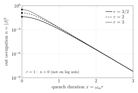
Exact occupation $n=|\beta|^2$ for the positive tanh frequency profile, plotted against $x=\omega_{\rm in}\tau$ at fixed $r=\omega_{\rm out}/\omega_{\rm in}=1.5,2,3$. The vertical axis is logarithmic; line styles distinguish the ratios. This is a quantitative oscillator calculation. The unchanged-frequency case $r=1$ has $n=0$ and is omitted from the logarithmic axis.

Representative values make the same comparison numerically:

$x$	$n$ for $r=1.5$	$n$ for $r=2$	$n$ for $r=3$
$0.1$	$0.03959175$	$0.1161850$	$0.2934320$
$0.5$	$0.01349039$	$0.02839246$	$0.04134981$
$1$	$0.001174023$	$0.001712735$	$0.001863955$
$2$	$3.192462\times10^{-6}$	$3.474342\times10^{-6}$	$3.487330\times10^{-6}$

Two limits independently check the interpretation. At fixed unequal positive frequencies, $\tau\to\infty$ gives $|\beta_k|^2\sim e^{-2\pi\tau\min(\omega_{k,\rm in},\omega_{k,\rm out})}$. Equal frequencies give exactly zero for every $\tau$. As $\tau\to0$,

$$|\beta_k|^2\longrightarrow \frac{(\omega_{k,\mathrm{out}}-\omega_{k,\mathrm{in}})^2} {4\omega_{k,\mathrm{out}}\omega_{k,\mathrm{in}}},$$

which is the sudden-oscillator matching result. Indeed, matching $u$ and $u'$ across a sudden jump gives $\beta=(\sqrt{\omega_{\rm out}/\omega_{\rm in}}-\sqrt{\omega_{\rm in}/\omega_{\rm out}})/2$. The exact companion coefficient has numerator $\sinh^2[\pi\tau(\omega_{\rm out}+\omega_{\rm in})/2]$ over the same denominator; subtracting the two squared coefficients gives one by a hyperbolic-function identity.

The sudden limit is modewise, not uniform in momentum. In the massive conformal FLRW realization, sudden matching gives $|\beta_k|^2\sim m^4(a_{\rm out}^2-a_{\rm in}^2)^2/(16k^4)$. Its three-dimensional number integral is ultraviolet finite, but its particle-energy integral has a logarithmic ultraviolet divergence. A smooth transition with nonzero $\tau$ suppresses that tail exponentially. This is why an exactly abrupt quench should not be used to infer a finite stress tensor for a smooth cosmology.

Particle number between the asymptotic eras

At finite $\eta$, the functions $\alpha_k(\eta)$ and $\beta_k(\eta)$ above refer to the specific zeroth-order instantaneous basis used in their definition. Replacing $\omega_k$ by a higher-order adiabatic frequency changes the instantaneous value, sometimes substantially near a nonadiabatic episode. Oscillatory transient terms are therefore not by themselves produced particles in an operationally invariant sense.

Late-time $|\beta_k|^2$ is stable when the out region supplies a genuine positive-frequency split. If the universe never becomes stationary, one should report the chosen adiabatic order, time, and basis, or compute a local observable such as a detector response or renormalized stress tensor. Adiabatic subtraction of the latter is a separate ultraviolet operation; it must not be confused with subtracting a particle number until it looks small. The relationship between adiabatic particles and stress-tensor regularization is developed in Parker and Fulling 1974, complete article, pp. 341–354.

The conformal no-creation check

For a massless conformally coupled scalar on a conformally flat FLRW patch,

$$m=0,\qquad \xi=\frac16,\qquad \omega_k=k.$$

The mixing source $\omega_k'/2\omega_k$ vanishes, hence $\beta_k=0$ for a state conformally transported from the Minkowski vacuum. The same check works for a massless Dirac field after the $a^{3/2}$ rescaling. The conclusion is not “expanding universes create no massless particles”: it requires a conformally invariant field, the conformal state, and compatible global and boundary conditions. A massless minimally coupled scalar has $\omega_k^2=k^2-a''/a$ and fails the check.

Diagnostic: interpret a transient occupation

During a smooth expansion, a zeroth-order adiabatic basis gives $|\beta_k(\eta_\ast)|^2=0.2$, while a fourth-order basis gives $0.03$ at the same intermediate time. Both tend to $0.05$ in a common stationary out region. Which value is a basis-independent particle prediction, and what two checks should accompany it?

Solution

Neither intermediate value is basis-independent; each is an instantaneous adiabatic occupation tied to a declared WKB convention. The shared late-time value $0.05$ is the out-particle prediction because the stationary region selects the same positive-frequency modes. One should verify the Wronskian identity $|\alpha_k|^2-|\beta_k|^2=1$ and the ultraviolet convergence of the integrated density. As an additional physics check, making the transition slower should suppress the final value, and the massless conformally coupled field in its conformal state should give zero.

References

• National Institute of Standards and Technology. n.d. Digital Library of Mathematical Functions, §§5.4 and 15.8, gamma-function identities and hypergeometric continuation. DLMF §5.4; DLMF §15.8.
• Parker, Leonard, and Stephen A. Fulling. “Adiabatic Regularization of the Energy-Momentum Tensor of a Quantized Field in Homogeneous Spaces.” Physical Review D 9 (1974): 341–354. DOI.
• Parker, Leonard. “Quantized Fields and Particle Creation in Expanding Universes. I.” Physical Review 183 (1969): 1057–1068. DOI.