Decoupling, Mass Scales, and Scheme Dependence

A heavy field admits a local curvature expansion only when every external geometric and boundary scale is small compared with its mass. At the evidence cutoff 2026-08-19, one-loop form factors give strong support for smooth infrared decoupling in curvature-squared response, but they do not justify an equally definite claim about the cosmological constant or Newton coupling. Minimal subtraction, momentum subtraction, and effective-field-theory matching describe different aspects of the same threshold and must not be compared as though their running couplings were observables.

Required background. Gravitational Actions and Boundary Terms provides the lower- and higher-derivative gravitational couplings and their boundary completion; Curvature supplies the curvature hierarchy. Helpful background. Flat-Spacetime Quantum Field Theory provides threshold matching and mass-dependent schemes; Partial Differential Equations and Green Functions supplies derivative expansions and spectral gaps; Causality and Global Structure establishes the Lorentzian regime and boundary scales; Quantum Fields in Curved Spacetime provides state, observable, and renormalization prescriptions.

The hierarchy behind the local large-mass expansion

For a Euclidean operator $D_m=D_0+m^2$, the proper-time integral contains $e^{-tm^2}$ and is dominated by $t\sim m^{-2}$. After the renormalized terms through $a_4$, the formal large-mass series has the structure

$$\Gamma_E^{(1)} \sim \Gamma_{\mathrm{local}}^{(0,2,4)} -\frac12\sum_{r=3}^{\infty} \frac{\Gamma(r-2)}{m^{2r-4}}\,a_{2r}(D_0).$$

Here $a_{2r}$ are the integrated coefficients including $(4\pi)^{-2}$, and the $-1/2$ and gamma function follow from integrating $-\tfrac12\int_0^\infty dt\,t^{r-3}e^{-tm^2}$. Thus the first omitted local terms are $-a_6/(2m^2)$ and $-a_8/(2m^4)$ with this Euclidean determinant convention. This derivative expansion requires, schematically,

$$\frac{|\mathcal R|}{m^2}\ll1, \qquad \frac{|\nabla\mathcal R|}{m^3}\ll1, \qquad \frac{|\nabla^2|}{m^2}\ll1,$$

for every curvature and background field entering the observable. With a boundary, extrinsic curvature, Robin coefficients, tangential momenta, and inverse distance to corners must satisfy analogous inequalities. A spectral gap and compatible boundary conditions are also needed. The expansion is asymptotic: truncating it can be controlled within a hierarchy, but convergence for arbitrary backgrounds is not promised.

The Euclidean coefficients translate into local Lorentzian operators only after the site’s $(-,+,+,+)$ continuation is fixed. They do not by themselves determine real-time particle production, an imaginary part, or a causal state-dependent kernel. Vassilevich distinguishes the ordinary and modified large-mass expansions from genuinely nonlocal resummations in Vassilevich 2003, §8.1, PDF.

Form factors interpolate between ultraviolet and infrared

At second order in curvature, a massive loop takes the covariant form

$$\Gamma_E^{(1)}\supset \frac{1}{2(4\pi)^2} \int d^4x\sqrt{g_E} \left[ \frac12C_{\mu\nu\rho\sigma} k_W(z)C^{\mu\nu\rho\sigma} +R_Ek_R(z)R_E \right],$$

where $z=-\nabla_E^2/m^2$. In the ultraviolet, $z\gg1$, the form factors contain logarithms. For a massive scalar, for example,

$$k_W(z)\sim-\frac1{60}\ln z+\cdots.$$

In the infrared, $z\ll1$, the same exact one-loop form factor is analytic,

$$k_W(z)\sim-\frac{z}{840}+O(z^2).$$

The corresponding mass-dependent beta function approaches its massless coefficient in the ultraviolet and is suppressed as $p^2/m^2$ in the infrared. Gorbar and Shapiro obtain explicitly

$$\beta_{C^2}^{\mathrm{IR}} =-\frac{1}{1680(4\pi)^2}\frac{p^2}{m^2} +O\!\left(\frac{p^4}{m^4}\right)$$

for their scalar normalization, with analogous smooth behavior for the $R^2$ sector Gorbar and Shapiro 2003, §§3–5, especially Eqs. (4.3)–(5.5), PDF. Their extension to scalars, fermions, and massive vectors confirms smooth higher-derivative thresholds while exposing field-dependent qualifications Gorbar and Shapiro 2003, Part II, §§3–5, PDF.

A resolved threshold between the two limits

The interpolation can be checked without extrapolating either asymptotic formula. For positive Euclidean $z=p^2/m^2$, the exact scalar form factor is

$$\begin{gathered} a=2\sqrt{\frac{z}{z+4}}, \qquad A=1-\frac{2}{a}\operatorname{artanh}\frac a2,\\ k_W(z)=\frac{8A}{15a^4}+\frac{2}{45a^2}+\frac1{150}. \end{gathered}$$

This is Gorbar and Shapiro 2003, Eqs. (3.5) and (3.7), PDF. The variable $a$ here is a form-factor parameter, not the trace-anomaly coefficient. At small $z$ the separate terms strongly cancel. An equivalent integral, obtained by integrating the logarithmic expression, makes numerical evaluation and the limiting behavior clearer:

$$k_W(z)=-\frac1{12}\int_0^1du\,(1-2u)^4 \log\bigl(1+zu(1-u)\bigr).$$

Normalize the mass-dependent response to its ultraviolet beta function, $\beta_{\mathrm{UV}}=-1/[120(4\pi)^2]$. Differentiation gives

$$\begin{aligned} B(z)&=\frac{\beta_{C^2}(z)}{\beta_{\mathrm{UV}}} =-60z\,\frac{dk_W}{dz}\\ &=5\int_0^1du\,(1-2u)^4 \frac{zu(1-u)}{1+zu(1-u)}. \end{aligned}$$

The integrand is positive and increases with $z$, while $5\int_0^1(1-2u)^4du=1$. Therefore $0\lt B(z)\lt1$ and $B$ increases monotonically to one. Expansion of the denominator gives $B(z)=z/14+O(z^2)$, in agreement with the source’s infrared beta function. Inspect how the curve follows this quadratic suppression well below the mass and gradually approaches its ultraviolet value; there is no abrupt switch at $p=m$.

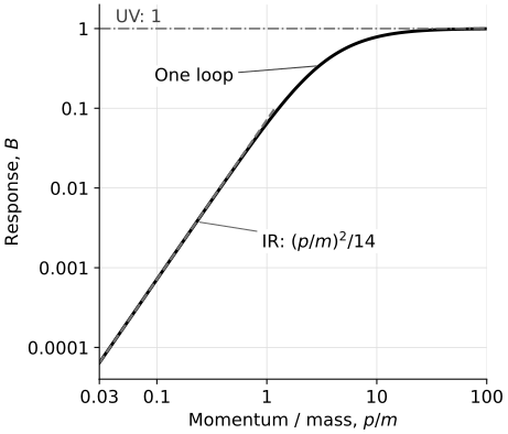
The normalized one-loop response $B=\beta_{C^2}/\beta_{\mathrm{UV}}$ for one real massive scalar, evaluated at positive Euclidean momentum in the weak-curvature expansion. Both axes are logarithmic. The solid curve is the integral above; the dashed low-momentum approximation is $(p/m)^2/14$, and the dash-dotted line is the ultraviolet limit. This is a quantitative form-factor calculation, not a claim about cosmological-constant or Newton-coupling running.

Representative values are $B=0.000713493$ at $p/m=0.1$, $0.0644314$ at $1$, $0.341470$ at $3$, $0.784154$ at $10$, and $0.993451$ at $100$. These also show that the ratio measures a scale-dependent response, not the abundance of real particles.

Competing positions are scheme statements

The credible competing positions concern what one calls “running.” In minimal subtraction, ultraviolet poles give mass-independent beta functions; a heavy field continues to appear below its mass unless one matches to a low-energy theory and removes it from the active spectrum. This is efficient for ultraviolet calculations but does not display a threshold automatically.

In a physical mass-dependent scheme, differentiation with respect to an external momentum or subtraction scale produces a smooth form factor and explicit $p^2/m^2$ suppression. The price is dependence on the chosen kinematics and observable. On a generic curved spacetime there is no unique global momentum, so the relevant scale may be an eigenvalue, curvature radius, frequency measured in a state, or a covariant operator argument.

Effective-field-theory matching integrates the heavy field out at a scale near $m$. Its effects remain in finite Wilson coefficients of local operators, while low-energy nonlocal propagation is generated only by light degrees of freedom. “Decoupled” therefore does not mean that every heavy-field contribution vanishes; it means that low-energy variations are power suppressed after matching, apart from renormalized local parameters.

Scheme dependence versus physical nonlocality

A finite counterterm

$$\Delta\Gamma=\alpha\int d^4x\sqrt{-g}\,C^2$$

shifts the constant part of $k_W(z)$. It does not change the logarithmic branch structure, threshold discontinuity, or a properly matched observable. Similarly, a finite $R^2$ term changes the local coefficient and the scheme-dependent $\Box R$ anomaly. Thus isolated values of gravitational couplings at one scale are not invariant predictions.

The separation must also respect boundaries. Bulk form factors do not determine finite boundary counterterms, and an integrated bulk total derivative can become a boundary response. A local expansion made on a closed Euclidean manifold cannot be transplanted unchanged to a Lorentzian region with reflecting or dissipative boundary data.

Results and limitations as of 2026-08-19

Position or result	Assumptions	Evidence	Limitation or adverse case
Local Schwinger–DeWitt expansion	$m^2$ dominates curvature, derivatives, boundary scales, and spectral gaps	Heat-kernel coefficients give a covariant series in inverse powers of $m^2$	Asymptotic and local; misses thresholds, homogeneous state data, and nonanalytic imaginary parts
Smooth higher-derivative decoupling	One loop, weak-curvature expansion through quadratic order, mass-dependent subtraction	Gorbar and Shapiro 2003, §§3–5, PDF find ultraviolet logs and infrared $p^2/m^2$ suppression	Directly supports $C^2$ and $R^2$ sectors, not arbitrary observables or nonperturbative backgrounds
Minimal-subtraction running	Dimensional regularization and ultraviolet pole subtraction	Correct ultraviolet coefficients and convenient covariant bookkeeping	Mass independent; threshold decoupling must be imposed through matching rather than read from the beta function
Cosmological and Newton sectors	Lower-derivative gravitational terms on curved backgrounds	The covariant divergences are known	Flat-background two-point form factors do not determine physical mass-dependent running; the infrared law remains unresolved
Massless anomaly action	Exactly massless conformal fields and chosen Green-function data	Vassilevich 2003, §9.1, PDF gives the nonlocal Polyakov example	It is an adverse case for extrapolating a local $1/m^2$ expansion to $m\to0$, where the hierarchy collapses

The evidence establishes controlled decoupling for specified form factors, not a theorem that every heavy field is irrelevant in every curved-spacetime observable. Confidence is high for the one-loop higher-derivative limits and lower for statements about $\Lambda$, $G$, strong curvature, horizons, time-dependent states, or interacting thresholds.

Failure modes and unresolved questions

The local hierarchy can fail even when a coordinate curvature component looks small. Large invariant tidal curvature, rapid time dependence, a nearly zero eigenvalue, a boundary layer of thickness $m^{-1}$, or an external frequency crossing $2m$ invalidates the Taylor expansion. Pair creation and tunneling terms can be exponentially small in the Euclidean asymptotic series yet carry the leading imaginary part of the Lorentzian action.

The most important unresolved discriminator is the lower-derivative sector. The flat-background polarization method makes momentum derivatives of the cosmological term vanish and turns the analogous Einstein insertion into a total derivative. Gorbar and Shapiro therefore state that their calculation does not determine mass-dependent beta functions for $\Lambda/G$ and $1/G$ Gorbar and Shapiro 2003, §5, pp. 15–17, PDF. A conjectured decoupling law there must be tied to a concrete curved-background observable, not inferred from the verified $C^2$ result.

Diagnostic: distinguish a threshold from a scheme shift

Suppose $k_W(z)=-z/840+O(z^2)$ for $z\ll1$ and $k_W(z)=-(1/60)\ln z+O(1)$ for $z\gg1$. What does each limit establish, and what changes after adding $\alpha\int\sqrt{-g}C^2$?

Solution

The infrared series shows that variations of the massive loop’s curvature-squared response are power suppressed by $p^2/m^2$ when the derivative expansion is valid. The ultraviolet logarithm reproduces the massless beta-function coefficient and signals nonlocal scale dependence. Adding the finite local $C^2$ counterterm shifts the $O(1)$ part of the form factor, so its quoted value at one subtraction point is scheme dependent. It changes neither the coefficient of the ultraviolet logarithm nor the existence of the smooth threshold in a matched observable. This check does not establish decoupling of the cosmological or Einstein terms, because those structures are not measured by the same quadratic form factor.

What could change these conclusions

The conclusions could change if a theorem or calculation extends mass-dependent decoupling to a new spacetime, state, boundary, algebra, or lower-derivative observable; if an independent reproduction changes either the ultraviolet logarithm or infrared $p^2/m^2$ coefficient; if a counterexample finds a nonanalytic low-energy term within the stated gapped regime; or if a regulator and matching analysis resolves the cosmological or Newton-sector ambiguity. New numerical or observational evidence is relevant only when it specifies the observable, state, curvature hierarchy, and renormalization prescription being compared.

References

• Gorbar, Eduard V., and Ilya L. Shapiro. “Renormalization Group and Decoupling in Curved Space: II. The Standard Model and Beyond.” Journal of High Energy Physics 2003, no. 06 (2003): 004. DOI. Open PDF.
• Gorbar, Eduard V., and Ilya L. Shapiro. “Renormalization Group and Decoupling in Curved Space.” Journal of High Energy Physics 2003, no. 02 (2003): 021. DOI. Open PDF, arXiv:hep-ph/0210388.
• Vassilevich, Dmitri V. “Heat Kernel Expansion: User’s Manual.” Physics Reports 388 (2003): 279–360. DOI. Open PDF, arXiv:hep-th/0306138.