Schwinger–Keldysh and In-In Dynamics

An expectation value at a finite time is an initial-value question: evolve the density operator and observable forward from the same initial state, then take a trace. An in-out functional answers a different question about a transition amplitude and generally supplies Feynman rather than retarded boundary data. The Schwinger–Keldysh closed-time path doubles fields and sources so that its physical limit yields normalized, real, causal in-in equations.

Required background. Flat-Spacetime Quantum Field Theory supplies source generating functionals and operator time ordering; Partial Differential Equations and Green Functions provides retarded initial-value response.

Helpful background. Causality and Global Structure establishes causal support on globally hyperbolic backgrounds; Quantum Fields in Curved Spacetime supplies the Hadamard initial-state condition and prescribed-metric setting.

The local bridge is the retarded solution rule. With $E=G_{\mathrm{ret}}-G_{\mathrm{adv}}$ and $[\Phi(f),\Phi(g)]=iE(f,g)\mathbf1$, a source perturbation can affect a later observable but not an earlier one. The doubled contour packages this support statement together with the density matrix and operator ordering.

The closed-time-path generating functional

Fix an initial Cauchy surface at $t_0$ and a normalized density operator $\rho_0$. Let $U_J(t_f,t_0)$ evolve with a source coupled through $S_J=S+\int J\phi\,d\mathrm{vol}_g$. Define

$$Z[J_+,J_-]=\operatorname{Tr}\!\left[ U_{J_+}(t_f,t_0)\rho_0 U_{J_-}(t_f,t_0)^\dagger \right].$$

The trace representation assumes a state normal in a chosen Hilbert-space representation, or a regulator where the density matrix exists. Algebraically the same expression is $\omega_0(U_{J_-}^\dagger U_{J_+})$. Its equal-source normalization follows from $\omega_0(\mathbf1)=1$, so the construction does not require a density matrix intrinsic to a sharp Type III local algebra. The path integral below is a perturbative representation, not a definition of a convergent continuum measure.

The plus branch runs from $t_0$ to a common return time $t_f$; the minus branch runs back. In a field basis, the same object is

$$\begin{aligned} Z[J_+,J_-]=\int &\mathcal D\phi_+\mathcal D\phi_-\, \rho_0(\phi_+^0,\phi_-^0)\\ &\times\exp\!\left\{iS[\phi_+]-iS[\phi_-] +i\int_M(J_+\phi_+-J_-\phi_-)d\mathrm{vol}_g\right\}, \end{aligned}$$

with $\phi_+(t_f)=\phi_-(t_f)$ integrated over. The minus signs are not optional decorations: they encode the adjoint backward evolution. Schwinger’s action-principle construction is the historical starting point Schwinger 1961, complete article, pp. 407–432, while Jordan develops effective equations for expectation values Jordan 1986, pp. 444–454.

The contour geometry below makes the endpoint matching and source doubling visible. Inspect the shared final endpoint: the path closes through the trace, not through a separately chosen out state.

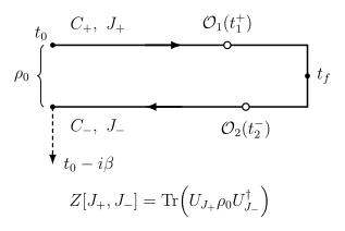
The in-in contour evolves from $t_0$ to the shared endpoint $t_f$ and back, with separate sources $J_\pm$ and operator insertions on the two branches. The initial state joins their initial data; the dashed leg is optional thermal preparation. Branch separation is schematic, not a separation of the physical return times.

The dashed leg to $t_0-i\beta$ represents $\rho_0\propto e^{-\beta H}$ when thermal preparation is intended. It is not required for an arbitrary nonequilibrium density matrix. The real-time branches, their matching condition, and the initial matrix element remain essential in either case.

Four propagators and the largest-time identity

For a bosonic field define

$$G^{ab}(x,y)=-i\langle T_C\phi_a(x)\phi_b(y)\rangle, \qquad a,b\in\{+,-\}.$$

Contour ordering gives

$$\begin{aligned} G^{++}(x,y)&=-i\langle T\phi(x)\phi(y)\rangle,\\ G^{--}(x,y)&=-i\langle \bar T\phi(x)\phi(y)\rangle,\\ G^{+-}(x,y)&=-i\langle \phi(y)\phi(x)\rangle\equiv G^<(x,y),\\ G^{-+}(x,y)&=-i\langle \phi(x)\phi(y)\rangle\equiv G^>(x,y). \end{aligned}$$

Expanding time ordering with step functions immediately yields

$$G^{++}+G^{--}=G^{+-}+G^{-+}.$$

This two-point relation is the simplest largest-time identity. In diagrams, the corresponding cancellations express unitarity when the latest vertex is summed over its two branch assignments. Chou and collaborators develop the matrix structure and real-time rules in Chou et al. 1985, complete review, pp. 1–131.

The coordinate $x^0$ below denotes a chosen global time function increasing toward the future. For spacelike-separated $x,y$, the commutator vanishes, so the retarded distribution does not depend on how that time function orders such points.

The retarded combination is

$$G_R(x,y)=G^{++}(x,y)-G^{+-}(x,y) =-i\theta(x^0-y^0)\langle[\phi(x),\phi(y)]\rangle.$$

For the free field and the site’s commutator convention, this equals $G_{\mathrm{ret}}(x,y)$. This is an exact normalization check: when $x$ is later than $y$, $E(x,y)=G_{\mathrm{ret}}(x,y)$, and $-i(iE)=E$.

Normalization and physical-source derivatives

If the two sources are equal, the forward and backward evolutions cancel inside the trace:

$$Z[J,J]=\operatorname{Tr}(U_J\rho_0U_J^\dagger) =\operatorname{Tr}\rho_0=1.$$

For $W=-i\ln Z$, it follows that $W[J,J]=0$. The branch derivatives agree up to the source sign,

$$\left.\frac{\delta W}{\delta J_+(x)}\right|_{J_+=J_-} =-\left.\frac{\delta W}{\delta J_-(x)}\right|_{J_+=J_-} =\langle\phi(x)\rangle_J.$$

Introduce average and difference fields

$$\phi_c=\frac{\phi_++\phi_-}{2},\qquad \phi_\Delta=\phi_+-\phi_-,$$

and similarly $J_c=(J_++J_-)/2$, $J_\Delta=J_+-J_-$. Then

$$J_+\phi_+-J_-\phi_-=J_\Delta\phi_c+J_c\phi_\Delta.$$

The physical limit is $J_\Delta=0$ and $\phi_\Delta=0$. Difference variables are nevertheless indispensable because varying with respect to them produces the physical equation.

Real and causal expectation equations

Let $\Gamma[\phi_c,\phi_\Delta]$ be the closed-time-path effective action. Unitarity and Hermiticity imply

$$\Gamma[\phi_c,0]=0, \qquad \Gamma[\phi_c,\phi_\Delta]^* =-\Gamma[\phi_c,-\phi_\Delta].$$

Consequently, the coefficient linear in $\phi_\Delta$ is real, while a quadratic noise kernel appears with an imaginary coefficient. The mean-field equation is

$$\left.\frac{\delta\Gamma}{\delta\phi_\Delta(x)}\right|_{\phi_\Delta=0}=0.$$

Its response kernels are retarded because the largest-time identities cancel future dependence. Calzetta and Hu exhibit this real, causal structure for curved-spacetime applications in Calzetta–Hu 1987, pp. 495–509.

There is a useful source-sign check. With $S_J=S+\int J\phi$, the free equation derived from the mostly-plus scalar action is $P\phi=-J$. Linear response is

$$\frac{\delta\langle\phi(x)\rangle}{\delta J(y)} =i\theta(x^0-y^0)\langle[\phi(x),\phi(y)]\rangle =-G_{\mathrm{ret}}(x,y),$$

which solves $P\,\delta\phi=-\delta J$. Choosing $S_J=S-\int J\phi$ reverses both signs. Causality is invariant, but comparing formulas without declaring the source convention is unsafe.

Why in-out data answer the wrong question

An in-out functional generates matrix elements such as

$$\frac{\langle\mathrm{out}|\phi(x)|\mathrm{in}\rangle} {\langle\mathrm{out}|\mathrm{in}\rangle},$$

not the expectation value $\operatorname{Tr}(\rho_0\phi(x))$ evolved from initial data. Its second variation contains the Feynman kernel, which mixes retarded and advanced support and may make an effective equation complex. That is appropriate for amplitudes with asymptotic boundary conditions, but not for a causal initial-value equation for a mean field.

Renormalization must respect the doubled structure. Bulk counterterms on the two branches are the same local covariant functionals with opposite action signs. An initial state with unacceptable ultraviolet singularities can also generate divergences localized on the initial surface, requiring state preparation or boundary counterterms; ordinary bulk renormalization does not cure that failure. The formalism remains on a prescribed metric unless a separate semiclassical or stochastic-gravity equation is supplied.

Solved diagnostic: verify normalization and response sign

Assume $\operatorname{Tr}\rho_0=1$, equal sources on both branches, $S_J=S+\int J\phi$, and $[\phi(x),\phi(y)]=iE(x,y)\mathbf1$. Show first that the generating functional is normalized and then determine the free response for $x$ in the causal future of $y$.

Solution

Equal sources give the same unitary on both branches, so cyclicity of the trace and unitarity yield $Z[J,J]=\operatorname{Tr}(U_J\rho_0U_J^\dagger)=\operatorname{Tr}\rho_0=1$. For the chosen positive action source, the Kubo derivative is $i\theta(x^0-y^0)\langle[\phi(x),\phi(y)]\rangle$. Substituting the commutator gives $-\theta(x^0-y^0)E(x,y)$. In the stated causal ordering, the advanced kernel vanishes and $E=G_{\mathrm{ret}}$, so the response is $-G_{\mathrm{ret}}$. This sign also follows by differentiating the classical equation $P\phi=-J$.

References

• Calzetta, Esteban, and B. L. Hu. “Closed-Time-Path Functional Formalism in Curved Spacetime: Application to Cosmological Back-Reaction Problems.” Physical Review D 35 (1987): 495–509. DOI.
• Chou, Kuang-chao, Zhao-bin Su, Bai-lin Hao, and Lu Yu. “Equilibrium and Nonequilibrium Formalisms Made Unified.” Physics Reports 118 (1985): 1–131. DOI.
• Jordan, R. D. “Effective Field Equations for Expectation Values.” Physical Review D 33 (1986): 444–454. DOI.
• Schwinger, Julian. “Brownian Motion of a Quantum Oscillator.” Journal of Mathematical Physics 2 (1961): 407–432. DOI.