Regge Calculus

Regge calculus represents a smooth metric by flat simplices joined along shared faces. Edge lengths determine each simplex geometry; curvature is absent inside a simplex and concentrated on codimension-two hinges. Parallel transport around a hinge rotates or boosts by its deficit angle, so hinge volume times deficit angle replaces the integrated scalar curvature. The construction gives exact discrete field equations on a fixed complex, while convergence and a quantum sum require additional assumptions.

Helpful background. Flat-Spacetime Quantum Field Theory supplies action and path-integral methods; Einstein Equations supplies the continuum equations; Quantum Information supplies finite-state language; Quantum Gravity supplies regulator distinctions; Causality and Global Structure supplies Lorentzian signature and boundaries; and Computational Relativity supplies mesh and residual checks.

Piecewise-flat metric data

Let $\mathcal T$ be a four-dimensional simplicial complex with a consistent Lorentzian assignment of squared edge lengths $s_e$. Every four-simplex must be nondegenerate with the declared signature, and neighboring simplices must induce the same metric on their common tetrahedron. In a Euclideanized local calculation one may use positive lengths $\ell_e$; a triangle with sides $\ell_1,\ell_2,\ell_3$ has area from Heron’s formula, and higher simplex volumes follow from the Cayley–Menger determinant Hamber 2009, ch. 4.

In four dimensions a hinge $h$ is a triangle. For an interior Euclidean hinge,

$$\epsilon_h=2\pi-\sum_{\sigma\supset h}\theta_h^\sigma,$$

where $\theta_h^\sigma$ is the interior dihedral angle in four-simplex $\sigma$. If the angles sum to $2\pi$, neighboring frames return unchanged around $h$ and the local complex is flat there. A nonzero deficit is the holonomy angle in the two-plane normal to $h$. Lorentzian hinges require oriented boost or rotation angles according to whether the normal plane is Lorentzian or Euclidean; one must not insert Euclidean angles into a Lorentzian action without a declared continuation.

Integrated curvature at a hinge

To derive the normalization without hiding Lorentzian angle choices, the equations in this section and the next use Euclidean flat simplices with positive edge lengths. Define the positive-sign curvature functional $I_{\mathrm R}$ below; the Euclidean action in the weight $e^{-S_E}$ is $S_E=-I_{\mathrm R}$. This overall sign leaves the stationary equations unchanged. A Lorentzian amplitude instead needs the causal hinge types and oriented boost angles described above; the Euclidean formula alone does not specify it.

Take a small two-surface transverse to $h$. It is a cone whose total angular defect is $\epsilon_h$. Since the geometry tangent to $h$ is flat, the curvature integral factorizes into hinge area and transverse defect:

$$\int_{\operatorname{star}(h)} d^4x\,\sqrt g\,R \longrightarrow 2A_h\epsilon_h.$$

The factor two converts sectional curvature in the normal plane to scalar curvature. Summing over hinges gives the four-dimensional curvature functional, including cosmological and boundary terms,

$$I_{\mathrm R}= \frac{1}{8\pi G} \left[ \sum_{h\subset\mathrm{interior}\,\mathcal T}A_h\epsilon_h +\sum_{h\subset\partial\mathcal T}A_h\psi_h -\Lambda\sum_{\sigma}V_\sigma \right].$$

Here $\psi_h=\pi-\sum_{\sigma\supset h}\theta_h^\sigma$ is the exterior angle at a Euclidean boundary hinge, the discrete analogue of the Gibbons–Hawking–York term with outward boundary orientation. For a locally flat boundary it vanishes. The relation between deficit holonomy and action is Regge’s central derivation Regge 1961, §§2–4.

Dimensions provide a direct check. In four dimensions $[A_h]=L^2$, $[G]=L^2$, $[\Lambda]=L^{-2}$, and $[V_\sigma]=L^4$, while angles are dimensionless. Every term in $I_{\mathrm R}$ is dimensionless.

Count the equilateral triangles in the two transverse sections below. The second drawing becomes a cone only after its marked radial edges are identified.

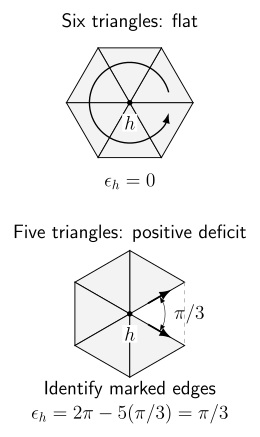
Six equilateral triangles give zero deficit. Five leave a gap of $\pi/3$; identifying the marked radial edges gives positive curvature at $h$. In four dimensions this is a section normal to a triangular hinge, with integrated scalar-curvature contribution $2A_h\epsilon_h$. Euclidean schematic; the cut is not a physical boundary and the drawn sectors are not four-simplices.

Discrete Einstein equations

Vary interior edge lengths while holding the induced boundary geometry fixed. Initially,

$$\delta\sum_h A_h\epsilon_h =\sum_h\epsilon_h\,\delta A_h +\sum_h A_h\,\delta\epsilon_h.$$

The flat-simplex Schläfli identity,

$$\sum_{h\subset\sigma}A_h\,\delta\theta_h^\sigma=0,$$

cancels the second sum after contributions are grouped simplex by simplex. Varying with respect to an interior length $\ell_e$ therefore gives

$$\boxed{ \sum_{h\supset e}\epsilon_h \frac{\partial A_h}{\partial\ell_e} -\Lambda\sum_{\sigma\supset e} \frac{\partial V_\sigma}{\partial\ell_e}=0. }$$

These are the Regge equations. They are invariant under relabeling the complex, but relabeling is a discrete symmetry and does not by itself generate the continuous gauge freedom of ADM theory. At flat configurations with $\Lambda=0$, admissible displacements of interior vertices can give exact Hessian null directions. Generic curved configurations lift these directions, so fixed-triangulation constraint counting must be performed for the chosen geometry and complex.

Limits and independent checks

Flat limit. If every interior deficit vanishes and $\Lambda=0$, the equations hold and transport around each hinge is trivial. This is necessary but not sufficient for a globally Euclidean geometry in the present derivation, or globally Minkowski geometry in its Lorentzian counterpart: topology and boundary identifications can retain global holonomy.

Two-dimensional limit. In two dimensions the hinges are vertices and the Regge curvature obeys

$$\int R\sqrt g\,d^2x=2\sum_v\epsilon_v.$$

For a closed triangulated surface, $\sum_v\epsilon_v=2\pi\chi$, so the action reproduces Gauss–Bonnet. This checks the factor of two and the deficit sign.

Refinement limit. Small deficits alone do not guarantee convergence: simplices can become skinny, signature constraints can fail, and different refinement sequences can represent different metrics. A trustworthy calculation monitors simplex quality, boundary data, equation residuals, and observables across multiple meshes. Regge’s original work establishes the discrete action and equations and discusses continuum approximation Regge 1961, §§4–5; it is not a general convergence theorem.

A quantum theory would additionally choose a measure over lengths or complexes, a contour or Lorentzian prescription, gauge factors, and renormalized observables. CDT fixes lengths and sums causal gluings; tensor models generate complexes combinatorially. Those are related but distinct dynamical definitions.

Exercises

At a vertex of a two-dimensional triangulation, $q$ equilateral triangles meet. Compute the deficit and integrated scalar curvature for $q=6$ and $q=5$. Explain the sign.

Solution

Each equilateral triangle contributes angle $\pi/3$, hence

$$\epsilon=2\pi-\frac{q\pi}{3}.$$

For $q=6$, $\epsilon=0$ and the neighborhood unfolds into a flat plane. For $q=5$, $\epsilon=\pi/3$, so the integrated scalar curvature assigned to the vertex is $2\epsilon=2\pi/3$. Removing one flat-plane wedge and identifying its edges produces a cone with positive curvature. If $q\gt6$, the deficit is negative and the cone is saddle-like in its intrinsic piecewise-flat sense.

References

• Hamber, Herbert W. Quantum Gravitation: The Feynman Path Integral Approach. Berlin: Springer, 2009. Publisher.
• Regge, Tullio. “General Relativity without Coordinates.” Nuovo Cimento 19 (1961): 558–571. DOI.