The Renormalized Semiclassical Field Equation

The renormalized semiclassical field equation determines a mean geometry only after more than a quantum state is chosen. One must also fix the field content, regulator and subtraction prescription, finite gravitational couplings at a scale, boundary or initial data, and the causal prescription for state response. With those inputs fixed, the equation equates a conserved local geometric variation to a conserved renormalized stress expectation; neither side is separately independent of finite scheme choices.

The renormalized expectation value is state dependent, while the local gravitational counterterms are not. The quantum state and renormalization prescription must therefore be stated together, with the renormalized couplings held to the same physical conditions. Keeping those two kinds of dependence distinct is part of the definition.

Required background. Einstein Equations supplies the classical tensor equation, and Gravitational Actions and Boundary Terms supplies the well-posed metric variation used to obtain its quantum-corrected form.

Helpful background. Quantum Fields in Curved Spacetime supplies Hadamard states and the renormalized stress expectation, while Black-Hole Geometry and Mechanics supplies later stationary boundary conditions.

The renormalized equation

Let $W_{\mathrm{ren}}[g^+,g^-;\rho]$ be the renormalized matter influence action on a closed time path with specified initial state $\rho$. The physical stress is the forward-branch derivative,

$$\langle T_{\mu\nu}\rangle_{\mathrm{ren}} =-\frac{2}{\sqrt{-g}} \left.\frac{\delta W_{\mathrm{ren}}}{\delta g_+^{\mu\nu}} \right|_{g^+=g^-=g}.$$

The branches are set equal after differentiation. Setting them equal first would give $W[g,g]=0$ by normalization and lose the response. For a four-derivative gravitational truncation, the field equation can be written

$$G_{\mu\nu}+\Lambda g_{\mu\nu} +16\pi G\left(\alpha H^{(R^2)}_{\mu\nu} +\beta H^{(C^2)}_{\mu\nu}\right) =8\pi G\,\langle T_{\mu\nu}\rangle_{\mathrm{ren}}.$$

Here $H^{(I)}_{\mu\nu}=(\sqrt{-g})^{-1}\delta I/\delta g^{\mu\nu}$, where $I$ is the integrated invariant, for example $I_{R^2}=\int d^4x\sqrt{-g}\,R^2$; this definition fixes the sign and normalization. The Euler-density and total-derivative terms have no independent local bulk variation in exactly four dimensions without boundaries, but they cannot be discarded blindly in dimensional regularization or boundary thermodynamics.

Hu and Verdaguer give this equation, with an equivalent curvature basis and source convention, in Hu and Verdaguer 2008, § 3.1, Eqs. (3.7)–(3.10). Their source convention is translated here to variation by $g^{\mu\nu}$ and the site’s $(-,+,+,+)$ curvature convention.

The data that must be fixed

The displayed formula is not a closed problem until the following are specified:

Input	Why it matters
geometry class and boundary or initial data	selects the gravitational solution space and required boundary terms
quantum fields and couplings	sets the effective action and anomaly coefficients
state or state-selection rule	fixes nonlocal polarization, flux, and regularity
regulator, subtraction, and scale $\mu$	defines the finite stress tensor and running couplings
$G(\mu),\Lambda(\mu),\alpha(\mu),\beta(\mu)$	supplies finite renormalization conditions
causal contour and approximation order	selects retarded response and the first omitted contribution

A Hadamard condition controls local ultraviolet singularities but does not uniquely select the state. A stationary boundary condition can select a vacuum in some spacetimes, while collapse or cosmology requires initial-state data. Conversely, the state cannot be chosen independently of a candidate geometry if regularity or self-consistency is required.

The arrows below show why all of these data belong to the same problem. In particular, follow the loop back to the geometry: computing the source on one metric does not establish that this metric solves its sourced equation.

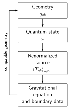
Geometry determines field evolution; the state and geometry determine the renormalized source, whose gravitational equation must yield a compatible metric. The field content, couplings, and state and boundary prescriptions are held fixed. Arrows show dependencies, not a proposed iteration or a proof of convergence. Schematic.

Derivation from the effective action

The physical equation follows by stationarity of the combined closed-time-path action,

$$\Gamma_{\mathrm{CTP}}[g^+,g^-] =S_{\mathrm{grav,ren}}[g^+]-S_{\mathrm{grav,ren}}[g^-] +W_{\mathrm{ren}}[g^+,g^-;\rho].$$

Vary the difference field $g^+_{\mu\nu}-g^-_{\mu\nu}$, impose the chosen initial density matrix and matching conditions, and set $g^+=g^-=g$ only after variation. This order yields a real causal expectation value. An in–out effective action instead computes transition amplitudes and can give a complex or acausal equation inappropriate for initial-value backreaction. Anderson, Molina-París, and Mottola explain the causal construction and its renormalized metric variation in Anderson, Molina-París, and Mottola 2003, §§ II–III, PDF.

Conservation and independent checks

Diffeomorphism invariance gives

$$\nabla^\mu\langle T_{\mu\nu}\rangle_{\mathrm{ren}}=0, \qquad \nabla^\mu H^{(R^2)}_{\mu\nu} =\nabla^\mu H^{(C^2)}_{\mu\nu}=0.$$

Together with $\nabla^\mu G_{\mu\nu}=0$, these identities make the equation consistent. They also detect noncovariant cutoffs, incomplete adiabatic subtraction, and numerical approximations that violate a Ward identity.

Dimensions supply a second check: every term scales as $L^{-2}$. In the limit $\alpha,\beta\to0$ and $\langle T_{\mu\nu}\rangle\to T^{\mathrm{class}}_{\mu\nu}$, the classical Einstein equation is recovered. Under a finite local scheme change, the matter and gravitational actions shift oppositely, so that their sum and the full field equation remain invariant. Since the stress tensor and geometric variation occur on opposite sides of the equation, their compensating tensor shifts have the same sign.

Predictive and excluded regimes

The equation predicts the mean metric only through the retained loop and derivative order. Higher derivatives can introduce spurious solutions if the truncation is treated as exact; stress fluctuations can invalidate the deterministic mean even when this equation has a smooth solution. Those issues are tested on later pages rather than hidden in the definition.

Fixed-background construction of $W_{\mathrm{ren}}$ remains in Quantum Fields in Curved Spacetime. Fine-grained information recovery and microscopic quantum-gravity dynamics are not determined by a conserved expectation-value source. They remain separate even when the semiclassical equation is solved exactly within its stated approximation.

Exercise

Suppose a finite prescription change adds $K_{\mu\nu}=aH^{(R^2)}_{\mu\nu}$ to $\langle T_{\mu\nu}\rangle_{\mathrm{ren}}$. Find the shift of $\alpha$ that leaves the displayed field equation unchanged.

Solution

Write the new equation using $T'_{\mu\nu}=T_{\mu\nu}+aH^{(R^2)}_{\mu\nu}$ and $\alpha'$. Its residual differs from the old one by

$$\left[16\pi G(\alpha'-\alpha)-8\pi Ga\right]H^{(R^2)}_{\mu\nu}.$$

It therefore vanishes for every metric when $\alpha'=\alpha+a/2$. A source shift $+aH^{(R^2)}$ arises from a matter-action shift $-a\int\sqrt{-g}R^2/2$, because the stress definition contains $-2$. Adding $+a\int\sqrt{-g}R^2/2$ to the gravitational action compensates it and gives the same answer. Merely moving the new source term left while holding $\alpha$ fixed would instead change the physical equation.

References

• Anderson, P. R., Molina-París, C., and Mottola, E. 2003. “Linear Response, Validity of Semi-Classical Gravity, and the Stability of Flat Space.” Physical Review D 67, 024026. Open PDF.
• Hu, B. L., and Verdaguer, E. 2008. “Stochastic Gravity: Theory and Applications.” Living Reviews in Relativity 11, 3. DOI.