Connection Forms and Cartan Structure Equations

Connection one-forms package covariant differentiation in a moving frame. Cartan’s first structure equation combines the coframe’s anholonomy with torsion; the second expresses curvature as the field strength of the connection. Together they turn many component-heavy calculations into exterior algebra while preserving every sign and index needed to reconstruct the Riemann tensor.

Required background. Pseudo-Riemannian Metrics and Signature supplies Lorentzian inner products and signature; Orthonormal Tetrads and Measured Components supplies orthonormal frames and coframes. Affine Connections and Covariant Derivatives supplies the general connection framework, The Levi-Civita Connection supplies the torsion-free metric specialization, and The Riemann Curvature Tensor fixes the adopted curvature commutator.

Helpful background. Calculus and Linear Algebra for Relativity supplies linear maps, basis changes, and index manipulations; Exterior Algebra and Differential Forms supplies forms and wedge products, while The Exterior Derivative and the Poincare Lemma supplies $d$. Killing Fields and Isometry Groups motivates adapted orthonormal frames.

Connection one-forms

For a frame $e_a$ with dual $\theta^a$, define the connection one-forms by

$$\nabla e_b=\omega^a{}_b\otimes e_a, \qquad \nabla_Xe_b=\omega^a{}_b(X)e_a.$$

Writing $\omega^a{}_b=\Gamma^a{}_{cb}\theta^c$ identifies their frame components with the connection coefficients. For an orthonormal frame and a metric-compatible connection,

$$\omega_{ab}=-\omega_{ba},$$

where the internal metric lowers the first frame index. In Lorentzian signature, that lowering includes the minus sign of the timelike leg; antisymmetry belongs to $\omega_{ab}$, not carelessly to every mixed-index matrix entry.

For a known orthonormal coframe, the torsion-free connection can be found without computing coordinate Christoffel symbols. First evaluate every $d\theta^a$, expand it in the wedge basis $\theta^b\wedge\theta^c$, impose $d\theta^a+\omega^a{}_b\wedge\theta^b=0$, and solve together with $\omega_{ab}=-\omega_{ba}$. Substitution back into all first-equation components is an important completeness check; solving only the visibly nonzero equation can miss allowed terms.

Carroll develops tetrads, spin connections, torsion, and curvature forms in Carroll 1997, §3, pp. 91–95, eqs. (3.130)–(3.143).

First structure equation

The torsion two-form is $T^a(X,Y)=\theta^a(T(X,Y))$. Expanding the definition $T(X,Y)=\nabla_XY-\nabla_YX-[X,Y]$ in the frame gives

$$T^a=d\theta^a+\omega^a{}_b\wedge\theta^b.$$

This is Cartan’s first structure equation. For the Levi-Civita connection, $T^a=0$, so the anholonomy of the coframe determines the antisymmetric part of the frame connection. If

$$d\theta^a=-\frac12 C^a{}_{bc}\theta^b\wedge\theta^c,$$

then setting torsion to zero relates $C^a{}_{bc}$ to the connection coefficients. Nonzero $d\theta^a$ therefore need not indicate torsion: it can be balanced exactly by $\omega^a{}_b\wedge\theta^b$.

Second structure equation

Apply two covariant derivatives to a frame vector. The curvature two-form is

$$\Omega^a{}_b =d\omega^a{}_b+\omega^a{}_c\wedge\omega^c{}_b =\frac12 R^a{}_{bcd}\theta^c\wedge\theta^d.$$

This is Cartan’s second structure equation. In a noncoordinate frame the precise commutator identity is

$$\left([\nabla_{e_c},\nabla_{e_d}] -C^f{}_{cd}\nabla_{e_f}\right)V =R(e_c,e_d)V.$$

The anholonomy term subtracts differentiation along $[e_c,e_d]$; omitting it would mistake noncommuting frame directions for curvature. In a coordinate frame $C^f{}_{cd}=0$, recovering the usual coordinate commutator. The quadratic term in $\Omega$ is matrix multiplication together with the wedge product; omitting it would also make curvature fail to transform covariantly under a changing frame.

The second equation follows by applying the connection twice. If a vector has frame components $v^a$, then $Dv^a=dv^a+\omega^a{}_b v^b$ and $D^2v^a=\Omega^a{}_b v^b$. This directly identifies the curvature form as the commutator of covariant derivatives in the frame representation. Expanding $\Omega^a{}_b$ in the coframe basis recovers every component of the Riemann tensor; no geometric information is lost by the form notation.

The exterior covariant derivative $D$ packages the Bianchi identities:

$$DT^a=\Omega^a{}_b\wedge\theta^b, \qquad D\Omega^a{}_b=0.$$

For zero torsion, the first reduces to $\Omega^a{}_b\wedge\theta^b=0$, equivalent to the algebraic Bianchi identity. The second is the differential Bianchi identity.

If torsion is allowed, one must not discard the $DT^a$ term or use the torsion-free algebraic identity unchanged. Cartan’s equations remain valid, but the connection is no longer fixed by the metric and coframe alone. The extra torsion data and their sign convention must be supplied explicitly.

Flat polar and curved-sphere checks

On the punctured Euclidean plane, take $\theta^1=dr$ and $\theta^2=r\,d\phi$. The torsion-free antisymmetric connection is

$$\omega^1{}_2=-d\phi, \qquad \omega^2{}_1=d\phi.$$

Indeed, $d\theta^2=dr\wedge d\phi$ is canceled by $\omega^2{}_1\wedge\theta^1=d\phi\wedge dr$. Yet

$$\Omega^1{}_2=d(-d\phi)=0$$

on the patch. The connection is nonzero because the orthonormal frame rotates; curvature is zero.

For a round two-sphere of radius $a$, use $\theta^1=a\,d\vartheta$ and $\theta^2=a\sin\vartheta\,d\phi$. The same torsion-free calculation gives

$$\omega^1{}_2=-\cos\vartheta\,d\phi,$$

and therefore

$$\Omega^1{}_2 =\sin\vartheta\,d\vartheta\wedge d\phi =\frac1{a^2}\theta^1\wedge\theta^2.$$

The polar plane and round sphere both have anholonomic orthonormal coframes, but only the sphere has nonzero curvature. This pair is a discriminating check on every term in both structure equations.

The two stacked calculations below make that distinction visible. Inspect the rotating frames and their nonzero connection forms in both panels, then compare the final curvature forms rather than inferring curvature from frame rotation alone.

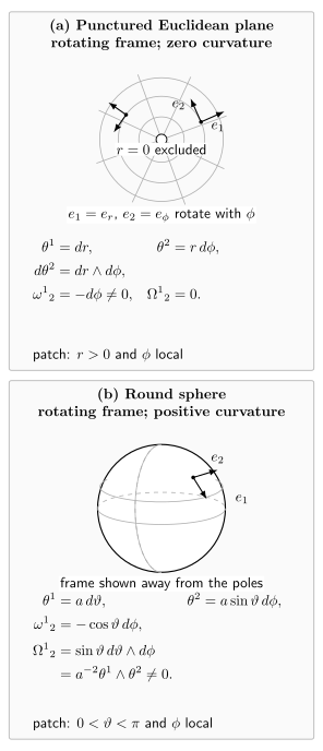
Both moving frames are anholonomic and have nonzero connection one-forms. Cartan’s second equation gives zero curvature in the punctured plane but $\Omega^1{}_2=a^{-2}\theta^1\wedge\theta^2$ on the sphere: nonzero connection coefficients do not imply curvature. Schematic comparison with exact formulas, away from the respective polar coordinate singularities.

Scope and calculation discipline

Connection forms are frame-dependent; curvature forms are frame-covariant. One may set a connection to zero at a point by a suitable local frame choice, but one cannot remove nonzero curvature there. Patch singularities such as $d\phi$ at a polar origin must not be confused with curvature.

For a practical sign check, reverse the orientation of the ordered coframe or interchange its two spatial legs and transform every indexed object consistently. Individual connection components change, but the reconstructed sectional curvature of the round sphere remains $1/a^2$. Changing one sign in isolation is not a convention change; it is an inconsistent calculation.

This page supplies geometric identities, not gravitational field equations or Newman–Penrose evolution equations. Any torsionful application must retain $T^a$ and state its convention explicitly rather than silently imposing the Levi-Civita case.

Exercises

Verify the round-sphere connection above from the first structure equation and compute the Gaussian curvature from the second.

Solution

Since $d\theta^1=0$ and $d\theta^2=a\cos\vartheta\,d\vartheta\wedge d\phi$, antisymmetry and $T^a=0$ are satisfied by $\omega^1{}_2=-\cos\vartheta\,d\phi$. Differentiating gives $\Omega^1{}_2=\sin\vartheta\,d\vartheta\wedge d\phi$. Because $\theta^1\wedge\theta^2=a^2\sin\vartheta\,d\vartheta\wedge d\phi$, the coefficient is $1/a^2$. In two dimensions that coefficient is the Gaussian curvature, positive and constant as expected.

References

• Carroll, Sean M. Lecture Notes on General Relativity. arXiv:gr-qc/9712019 (1997), arXiv.