Foliations, Lapse, and Shift

A spacelike foliation writes a spacetime region as a one-parameter family of spacelike hypersurfaces. The lapse tells how much proper time separates neighboring slices along their future unit normals; the shift tells how the spatial coordinates slide tangentially from one slice to the next. Together with the induced metric they reconstruct the spacetime metric kinematically.

Because the construction is geometric, one can change adapted coordinates and obtain different lapse and shift while preserving the same foliation and spacetime metric; their transformation must be followed together with the coordinate labels.

The split separates three choices that are often blended together: which hypersurfaces count as equal time, how quickly the time label advances between them, and how spatial points are identified from one slice to the next. The first fixes the normal direction, the lapse normalizes the label rate, and the shift fixes the tangential identification. None of these choices should be mistaken for an observable flow without an additional physical specification.

Required background. Affine Connections and Covariant Derivatives supplies covariant differentiation, while Flows and Lie Derivatives supplies the flow-based derivative used for evolution; The Riemann Curvature Tensor supplies later curvature projections; Pseudo-Riemannian Metrics and Signature supplies spacelike slices and timelike normals. Helpful background. Calculus and Linear Algebra for Relativity supplies block decompositions; Exterior Algebra and Differential Forms supplies the form and pullback language used for level-set time functions.

Time function and evolution vector

Let $t$ be a smooth time function whose level sets $\Sigma_t$ are spacelike. Their future-directed unit normal can be written

$$n_\mu=-N\nabla_\mu t, \qquad N>0,$$

where normalization gives

$$N=\left(-g^{\mu\nu}\nabla_\mu t\nabla_\nu t\right)^{-1/2}.$$

Choose coordinates $x^i$ on one slice and propagate their labels so that the coordinate evolution vector is $t^\mu=(\partial/\partial t)^\mu$. Since $t^\mu\nabla_\mu t=1$ and $n^\mu\nabla_\mu t=1/N$, the unique normal–tangential split is

$$t^\mu=Nn^\mu+\beta^\mu, \qquad n_\mu\beta^\mu=0.$$

The lapse $N$ is a scalar on each slice. The shift $\beta^\mu$ is a tangential vector. Neither is determined by the intrinsic metric alone; both describe how the foliation and coordinate labels are threaded through spacetime.

The vector triangle below makes the two roles geometrically distinct. Follow the normal leg from the lower leaf, then the tangential leg within the upper leaf, and compare their sum with the coordinate-time displacement.

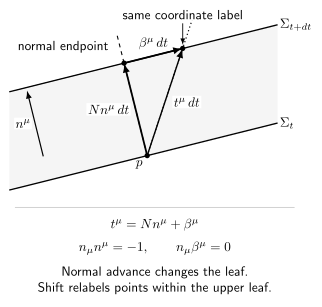
A coordinate-time displacement is the sum of normal proper advance N n dt and tangential coordinate shift beta dt. A coordinate line is normal only when the shift vanishes. Schematic and not to scale.

Reconstructing the line element

In coordinates adapted to the foliation,

$$ds^2 =-N^2dt^2 +h_{ij}(dx^i+\beta^i dt)(dx^j+\beta^j dt).$$

Thus

$$g_{tt}=-N^2+h_{ij}\beta^i\beta^j, \qquad g_{ti}=h_{ij}\beta^j, \qquad g_{ij}=h_{ij}.$$

The inverse components are

$$g^{tt}=-\frac1{N^2}, \qquad g^{ti}=\frac{\beta^i}{N^2}, \qquad g^{ij}=h^{ij}-\frac{\beta^i\beta^j}{N^2}.$$

Multiplying the two block matrices verifies these expressions. The determinant satisfies $\sqrt{-g}=N\sqrt h$. These algebraic checks catch the common mistake of omitting the shift-squared term in $g_{tt}$.

The spacetime volume element consequently factors as normal proper separation times spatial volume:

$$dV_g=N\,dt\,dV_h.$$

This factorization is local and orientation sensitive. It is useful for integrals over a foliated region, but it does not assert that the coordinates cover the entire spacetime or that all slices are complete.

Metric change and normal acceleration

Using the convention

$$K_{ij} =-h_i{}^\mu h_j{}^\nu\nabla_\mu n_\nu,$$

the normal derivative of the spatial metric is $\mathcal L_nh_{ij}=-2K_{ij}$. Because $t^\mu=Nn^\mu+\beta^\mu$,

$$\partial_t h_{ij} =-2NK_{ij}+\mathcal L_\beta h_{ij},$$

or

$$K_{ij} =-\frac1{2N} \left(\partial_t h_{ij}-\mathcal L_\beta h_{ij}\right).$$

This identity says how the embedding changes under the chosen threading. It does not prescribe dynamics for $h_{ij}$.

The normal congruence generally accelerates. Projection of its derivative gives

$$a_i=h_i{}^\mu n^\nu\nabla_\nu n_\mu=D_i\ln N.$$

A lapse constant on each slice makes the normal curves geodesic, although it may still vary from slice to slice. The shift does not enter this invariant acceleration; it changes coordinate threading rather than the normal itself. These relations are derived in Gourgoulhon 2007, §3.3, pp. 41–46 and §4.2, pp. 54–59.

Flat-spacetime checks

Cartesian Minkowski slicing has $N=1$, $\beta^i=0$, time-independent $h_{ij}$, and hence $K_{ij}=0$. The same spacetime in uniformly translated spatial coordinates has a nonzero constant shift, but $\mathcal L_\beta h=0$ and $K$ remains zero.

Milne coordinates inside the future cone have

$$ds^2=-d\tau^2+\tau^2\gamma_{ij}dx^idx^j.$$

Here $N=1$, $\beta=0$, and

$$K_{ij}=-\frac12\partial_\tau h_{ij} =-\frac1\tau h_{ij}.$$

This is an essential check: extrinsic curvature depends on the slicing even when the ambient Riemann tensor vanishes.

Rindler slicing,

$$ds^2=-\rho^2d\eta^2+d\rho^2+dy^2+dz^2,$$

has $N=\rho$, zero shift, and time-independent spatial metric, so $K_{ij}=0$ while $a_\rho=D_\rho\ln\rho=1/\rho$. This distinguishes acceleration of the normals from bending of the slices.

The decomposition may fail globally even when it works locally. A time function can cease to have spacelike level sets, a lapse can approach zero at a coordinate boundary, or normal curves can intersect. These are failures of a selected foliation or adapted chart unless an independent invariant diagnosis establishes something stronger.

Common pitfalls

Lapse is not generally proper time per coordinate time for every worldline. The statement applies along the normal displacement between slices. A coordinate line with nonzero shift is not normal.

Shift is not a spacetime vector independent of the foliation. It is the tangential part of the selected evolution field. Changing spatial coordinates changes its components and may change the field itself.

The metric-change equation is kinematic. Constraints, gauge choices for evolution, and numerical formulations require gravitational dynamics and lie outside this page.

Exercises

Starting from the reconstructed line element, derive the future unit normal components in adapted coordinates.

Solution

Because $n_\mu=-N\nabla_\mu t$,

$$n_\mu=(-N,0,0,0).$$

Raising with the inverse metric gives

$$n^t=\frac1N, \qquad n^i=-\frac{\beta^i}{N}.$$

Then $n^\mu n_\mu=-1$, and

$$\partial_t=Nn+\beta$$

follows component by component. This verifies both the shift sign in the line element and the normalization of the lapse.

References

• Gourgoulhon, Éric. 3+1 Formalism and Bases of Numerical Relativity. Lecture notes, 2007. arXiv:gr-qc/0703035.