Parallel Transport Along Curves

Parallel transport is the connection’s rule for carrying a vector along a specified curve while declaring its covariant derivative to vanish. It is a linear initial-value problem, so it produces an invertible map between the endpoint tangent spaces. Dependence of that map on the chosen path is holonomy: it records geometric information that no comparison of coordinate components at separated points can supply.

Required background. Tensor Fields and Natural Operations supplies vector fields along curves and changes of frame; Pseudo-Riemannian Metrics and Signature supplies inner products whose preservation requires metric compatibility.

Helpful background. Calculus and Linear Algebra for Relativity supplies linear ordinary differential equations and uniqueness of initial-value problems.

Parallel fields as an ODE

Let $\gamma:I\to M$ be a smooth curve with parameter $\lambda$. A vector field $V$ along $\gamma$ is parallel when

$$\frac{DV}{d\lambda} \equiv\nabla_{\dot\gamma}V=0.$$

In coordinates this is the linear system

$$\frac{dV^\rho}{d\lambda} +\dot x^\mu\Gamma^\rho{}_{\mu\nu}(x(\lambda))V^\nu=0.$$

For a smooth connection and a fixed initial value $V(\lambda_0)=v\in T_{\gamma(\lambda_0)}M$, standard ODE theory gives a unique solution over every interval on which the curve and coefficients remain defined. It therefore defines a linear transport map

$$P^\gamma_{\lambda_0\to\lambda_1}: T_{\gamma(\lambda_0)}M\longrightarrow T_{\gamma(\lambda_1)}M.$$

Uniqueness immediately yields

$$P_{\lambda\to\lambda}=\operatorname{id}, \qquad P_{\lambda_1\to\lambda_2}P_{\lambda_0\to\lambda_1} =P_{\lambda_0\to\lambda_2}, \qquad \left(P_{\lambda_0\to\lambda_1}\right)^{-1} =P_{\lambda_1\to\lambda_0}.$$

The last map uses the reversed curve. Under an orientation-preserving reparametrization $\lambda=\lambda(s)$, both terms in the transport equation acquire the same factor:

$$\frac{DV}{ds}=\frac{d\lambda}{ds}\frac{DV}{d\lambda}.$$

Thus the zero-derivative condition and the transport map are unchanged.

Calegari develops parallel transport as a connection ODE in Calegari 2022, §5.2, pp. 42–43, PDF.

Metric preservation is an extra condition

Suppose $V$ and $W$ are parallel along $\gamma$. Then

$$\frac{d}{d\lambda}g(V,W) =(\nabla_{\dot\gamma}g)(V,W).$$

Consequently a metric-compatible connection, $\nabla g=0$, transports inner products, norms, causal characters, and angles unchanged. An arbitrary affine connection need not do so. Parallel transport is defined before a metric is chosen, and even after a metric is chosen, preservation follows only when nonmetricity vanishes.

Transport also acts on covectors and tensors using the induced connection. Because contractions commute with covariant differentiation, pairing a parallel covector with a parallel vector gives a constant scalar. These facts make transport a comparison map for every tensor type, not merely for arrows drawn in a coordinate chart.

A spherical-loop calculation

On the unit two-sphere with its Levi-Civita connection, consider a geodesic triangle: travel from the north pole down the longitude $\phi=0$ to the equator, along the equator through angle $\alpha$, and back to the north pole along longitude $\phi=\alpha$, where $0\lt\alpha\lt\pi$. Give the sphere its outward orientation; this traversal positively orients the triangle’s boundary.

Start with the vector tangent to the first meridian. Along that great circle, its parallel transport remains the tangent. At the first equatorial vertex it is the constant ambient vector $-\partial_z$. This vector is tangent to the sphere all along the equator, and its ordinary derivative in $\mathbb R^3$ vanishes, so its tangential covariant derivative also vanishes. At the second vertex it is opposite to the tangent of the return meridian and remains so along that great circle.

Back at the north pole, the transported vector points along longitude $\phi=\alpha$, whereas the initial vector pointed along $\phi=0$. The loop has rotated it through angle $\alpha$. The result depends on the path even though the starting and ending point are identical. It also equals the area $\alpha$ of this unit-sphere triangle, anticipating the curvature–holonomy relation developed in the next chapter.

The diagram below separates the curved-space loop from its linear return map. Follow the three traversal arrows on the sphere, then compare the two arrows in $T_NS^2$; reversing the traversal reverses the signed rotation without changing the enclosed unsigned area.

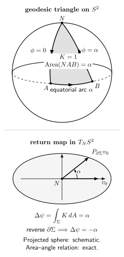
Parallel transport around the geodesic triangle returns the tangent vector rotated by the signed spherical area, which is $\alpha$ on the unit sphere. Reversing the traversal reverses the rotation. Schematic projection; the angle and area relation is exact.

Holonomy and what path dependence means

Transport around a loop based at $p$ is an automorphism of $T_pM$. The group generated by all such maps is the holonomy group at $p$. Small-loop dependence is controlled by curvature; see Tong 2019, §3.3.3, pp. 123–127, PDF. The current page uses it only as an interpretation, not as a curvature classification.

Several qualifications matter. Open-path transport cannot be compared across two paths until their endpoints and initial vector are fixed. A flat connection on a simply connected region has path-independent transport, but a flat connection on a non-simply-connected space or bundle can retain global holonomy. The reason is that flatness makes transport invariant under a deformation of the path with endpoints fixed, whereas noncontractible loops need not deform to the constant loop; see Calegari 2022, §4.3, p. 33, PDF. Torsion is not identical to loop holonomy, and nonmetricity can change lengths even along an open path.

A parallel frame along one selected curve makes its directional connection coefficients vanish, yet transport around other curves can remain nontrivial. This does not make all connection coefficients vanish in a neighborhood. Conversely, nonzero coefficients in polar coordinates do not imply path dependence: flat Euclidean transport returns every vector unchanged around a contractible loop. The invariant object is the resulting map, not the intermediate components.

Exercises

Let $\gamma=\gamma_2*\gamma_1$ first traverse $\gamma_1$ from $p$ to $q$ and then $\gamma_2$ from $q$ to $r$. Prove from uniqueness of the transport ODE that $P^\gamma_{p\to r}=P^{\gamma_2}_{q\to r}P^{\gamma_1}_{p\to q}$, and use the reversed curve to prove invertibility.

Solution

Transport an initial vector $v$ along $\gamma_1$, obtaining $w=P^{\gamma_1}_{p\to q}v$, and then solve the same parallel equation along $\gamma_2$ with initial value $w$. The concatenated field is parallel on both pieces and has initial value $v$. By uniqueness it is the parallel field along $\gamma$, which proves the composition law. Transporting the result back along the reversed curve solves the original ODE backward and returns $v$, so reverse transport is the inverse map.

Repeat the spherical-loop calculation on a sphere of radius $a$. Without solving the transport ODE again, determine the rotation angle for the same triangle, check it against $K\operatorname{Area}(\Sigma)$, and state what happens when the loop orientation is reversed. Contrast the result with Levi-Civita transport around a triangle in the Euclidean plane.

Solution

Rescaling the sphere changes lengths but not the angles between the two meridians and the equator, so the transported vector again rotates through angle $\alpha$. Equivalently, the sphere has Gaussian curvature $K=1/a^2$ and the geodesic triangle has area $a^2\alpha$, hence

$$K\operatorname{Area}(\Sigma) =\frac{1}{a^2}(a^2\alpha)=\alpha.$$

With the orientation of the worked loop declared positive, the signed angle is $+\alpha$. Reversing the loop replaces the transport map by its inverse and therefore changes the signed angle to $-\alpha$. In the Euclidean plane, parallel vector components in Cartesian coordinates are constant and the curvature is zero, so transport around any triangle returns the vector with zero rotation. The comparison separates a coordinate description of the path from the invariant holonomy map.

References

• Calegari, Danny. Introduction to Differential Geometry. Preliminary version, May 26, 2022, University of Chicago, §4.3, p. 33, and §5.2, pp. 42–43. Course PDF.
• Tong, David. General Relativity. University of Cambridge lecture notes, 2019, §3.3.3, pp. 123–127. Official course PDF.