Presymplectic Potentials and Currents

A varied Lagrangian produces a boundary potential, and antisymmetrizing a second variation produces a current on spacetime. Integrating that current over a hypersurface gives a two-form on the space of solutions. It is called presymplectic because gauge transformations can lie in its kernel. The construction is local and covariant, but its conservation, boundary independence, and degeneracies hold only under explicit equations, linearized equations, and boundary-flux conditions.

Required background. Exterior Algebra and Differential Forms supplies spacetime forms and graded products; the Exterior Derivative and Poincaré Lemma supplies exact-form ambiguities, and the generalized Stokes theorem supplies the boundary identity. Tensor Fields and Natural Operations supplies smooth tensor fields and their algebraic operations; field variations are defined earlier in this chapter.

Helpful background. Calculus and Linear Algebra supplies antisymmetric bilinear forms and integration by parts; Variational Mechanics and Symmetries supplies canonical momenta and the finite-dimensional model.

From the potential to the current

Let an $n$-form Lagrangian satisfy

$$\boldsymbol\delta\mathbf L =\mathbf E_A\boldsymbol\delta\phi^A+d\boldsymbol\Theta(\phi;\boldsymbol\delta\phi).$$

For commuting variations $\delta_1$ and $\delta_2$, adopt the Iyer–Wald sign convention

$$\boldsymbol\omega(\phi;\delta_1\phi,\delta_2\phi) =\delta_2\boldsymbol\Theta(\phi;\delta_1\phi) -\delta_1\boldsymbol\Theta(\phi;\delta_2\phi).$$

This is a spacetime $(n-1)$-form and an antisymmetric field-space two-form. For field-dependent variation vectors, the same convention reads

$$\boldsymbol\omega(\delta_1,\delta_2) =\delta_2\boldsymbol\Theta(\delta_1) -\delta_1\boldsymbol\Theta(\delta_2) +\boldsymbol\Theta([\delta_1,\delta_2]) =-\boldsymbol\delta\boldsymbol\Theta(\delta_1,\delta_2).$$

The bracket term is therefore required, not optional: it is what makes the current a genuine field-space exterior derivative. The Lagrangian decomposition and symplectic-current definition appear in Iyer and Wald 1994, §3, Eqs. (20) and (44), pp. 6 and 9 of the preprint, PDF.

Apply $\delta_1\delta_2-\delta_2\delta_1$ to the varied Lagrangian. Since ordinary variations commute on $\mathbf L$, one obtains schematically

$$d\boldsymbol\omega =\delta_1\mathbf E_A\,\delta_2\phi^A -\delta_2\mathbf E_A\,\delta_1\phi^A.$$

Therefore $d\boldsymbol\omega=0$ when the background solves $\mathbf E_A=0$ and both tangent vectors solve the linearized equations. Merely putting the background on shell is not enough. This is the independent closure check: the antisymmetrized second variation cancels the second derivatives of the action, leaving precisely the linearized equations.

Scalar-field current and its check

For the fixed-background scalar Lagrangian

$$\mathbf L=-\frac12d\phi\wedge\star d\phi-V(\phi)\varepsilon,$$

one may take $\boldsymbol\Theta=-\boldsymbol\delta\phi\,\star d\phi$. The current becomes

$$\boldsymbol\omega(\delta_1,\delta_2) =\delta_2\phi\,\star d\delta_1\phi -\delta_1\phi\,\star d\delta_2\phi.$$

Its exterior derivative is

$$d\boldsymbol\omega =\left(\delta_2\phi\,\mathcal J\delta_1\phi -\delta_1\phi\,\mathcal J\delta_2\phi\right)\varepsilon,$$

where $\mathcal J=\Box-V''(\phi)$ is the linearized scalar operator. Hence the current is closed for two linearized solutions. The check also exposes the hypotheses: the metric and Hodge operator were held fixed, and smoothness was sufficient for integration by parts.

For an oriented hypersurface $\Sigma$, define

$$\Omega_\Sigma(\delta_1,\delta_2)=\int_\Sigma\boldsymbol\omega(\delta_1,\delta_2).$$

If a region $U$ has oriented boundary $\partial U=\Sigma_2-\Sigma_1+\mathcal B$, Stokes’ theorem gives

$$\Omega_{\Sigma_2}-\Omega_{\Sigma_1} =\int_Ud\boldsymbol\omega-\int_{\mathcal B}\boldsymbol\omega,$$

with the sign of the side boundary $\mathcal B$ fixed by outward-normal-first orientation. On linearized solutions, hypersurface independence still requires zero flux through $\mathcal B$. Conservation is thus a statement about equations plus boundary conditions, not a consequence of notation alone.

Ambiguities and surface sensitivity

Two standard ambiguities must be tracked together:

$$\mathbf L\mapsto\mathbf L+d\boldsymbol\mu, \qquad \boldsymbol\Theta\mapsto \boldsymbol\Theta+\boldsymbol\delta\boldsymbol\mu+d\mathbf Y.$$

Because $\boldsymbol\delta^2=0$, the $\boldsymbol\mu$ term drops out of the antisymmetrized current. The $\mathbf Y$ term changes it by a spacetime exact form,

$$\boldsymbol\omega\mapsto \boldsymbol\omega+d\!\left[ \delta_2\mathbf Y(\delta_1)-\delta_1\mathbf Y(\delta_2) \right].$$

This display uses commuting variations; for field-dependent ones add the corresponding $\mathbf Y([\delta_1,\delta_2])$ term inside the brackets. The exact change leaves an integral over a closed $\Sigma$ unchanged but can shift an integral when $\partial\Sigma\ne\varnothing$. Iyer and Wald state the corresponding Lagrangian and potential ambiguities in Iyer and Wald 1994, §3, Eqs. (40)–(43), p. 9 of the preprint, PDF. Boundary counterterms, corner choices, and falloff conditions must be fixed before a surface quantity is assigned. Harlow and Wu analyze the compatible boundary variational principle and these surface effects in Harlow and Wu 2020, §2.2, Eqs. (2.20)–(2.24), pp. 13–14.

Why the form is pre-symplectic

A closed two-form is symplectic only if its kernel vanishes. Gauge variations often satisfy

$$\Omega_\Sigma(\delta\phi,\delta_\lambda\phi)=0$$

for every admissible $\delta\phi$, making $\delta_\lambda\phi$ a degeneracy. But this conclusion depends on whether the gauge parameter obeys the boundary conditions and whether the associated surface term vanishes. A transformation with nonzero boundary action may instead generate a genuine symmetry. A boundary by itself neither proves nor disproves the existence of physical boundary degrees of freedom.

This kernel test is distinct from the side-boundary flux test. Zero flux makes $\Omega_\Sigma$ independent of the chosen hypersurface; it does not force every admissible boundary transformation into its kernel. A transformation can have a nonzero pairing and a conserved surface charge even when the flux vanishes. Conversely, nonzero flux establishes hypersurface dependence of the proposed $\Omega_\Sigma$, not the existence of a charged symmetry. Calling a nondegenerate boundary transformation Hamiltonian additionally requires its contraction with $\Omega_\Sigma$ to be the variation of a well-defined charge. A compatible boundary contribution can sometimes cancel flux, but that enlarged variational problem must be specified.

The formal solution space may also be singular, the quotient may fail to be a manifold, and the integral may diverge without falloff conditions. This page supplies the differential-geometric construction, not a functional-analytic existence theorem or a definition of gravitational charge.

The diagram below separates these tests. Read downward along the central chain, then compare the side branches: nonzero boundary flux interrupts hypersurface independence, whereas a nonzero pairing with an admissible transformation prevents quotienting that transformation as a kernel direction.

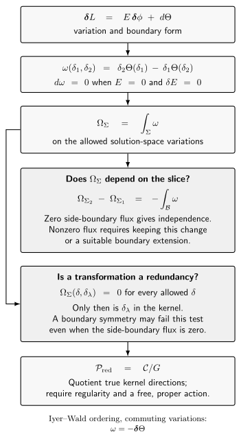
A boundary potential does not automatically produce a conserved symplectic form or a quotient phase space. Equations, linearized equations, boundary-flux conditions, kernel tests, and quotient regularity enter at distinct stages. With $\partial U=\Sigma_2-\Sigma_1+\mathcal B$, on-shell closure gives $\Omega_{\Sigma_2}-\Omega_{\Sigma_1}=-\int_{\mathcal B}\boldsymbol\omega$. Flux controls hypersurface dependence; the pairing with a transformation decides whether it is a kernel direction. A surface symmetry and its charge require a separate admissibility and integrability analysis. Schematic process diagram.

Exercise: Klein–Gordon flux

Let $\delta_1\phi$ and $\delta_2\phi$ satisfy $(\Box-m^2)\delta_i\phi=0$ on a fixed background. Show directly that the scalar presymplectic current is closed and state when its integrals over two hypersurfaces agree.

Solution

Using the current above,

$$d\boldsymbol\omega =\left[ \delta_2\phi(\Box-m^2)\delta_1\phi -\delta_1\phi(\Box-m^2)\delta_2\phi \right]\varepsilon=0.$$

For a region bounded by $\Sigma_1$, $\Sigma_2$, and a side boundary $\mathcal B$, Stokes’ theorem gives $\Omega_{\Sigma_2}-\Omega_{\Sigma_1}=-\int_{\mathcal B}\boldsymbol\omega$. The two integrals agree if the boundary conditions or falloff make this flux vanish. Closure alone is insufficient when a side boundary is present.

References

• Harlow, Daniel, and Jie-qiang Wu. “Covariant Phase Space with Boundaries.” Journal of High Energy Physics 10 (2020), 146. DOI; Open PDF.
• Iyer, Vivek, and Robert M. Wald. “Some Properties of Noether Charge and a Proposal for Dynamical Black Hole Entropy.” Physical Review D 50 (1994): 846–864. DOI.