Smooth Manifolds and Coordinate Atlases

A smooth manifold is a space that can be calculated on locally with ordinary coordinates while retaining a coordinate-independent notion of smoothness. The decisive condition is not that one preferred coordinate system exists, but that every overlap map between accepted charts is smooth. This page makes that condition explicit, checks it on the two stereographic charts of $S^2$, and explains the separation assumptions that prevent locally Euclidean spaces from developing pathological global behavior.

Required background. Calculus and Linear Algebra for Relativity — use multivariable derivatives, invertible Jacobians, and compositions of maps between Euclidean spaces.

Topological manifolds and smooth atlases

An $n$-dimensional topological manifold is a Hausdorff, second-countable topological space $M$ in which every point has a neighborhood homeomorphic to an open subset of $\mathbb R^n$. A chart is such a homeomorphism

$$\varphi_\alpha:U_\alpha\longrightarrow \varphi_\alpha(U_\alpha)\subset\mathbb R^n,$$

and the component functions $x^1,\ldots,x^n$ of $\varphi_\alpha$ are coordinates. An atlas covers $M$ by chart domains. Two charts are smoothly compatible when, wherever they overlap, the transition map

$$\varphi_\beta\circ\varphi_\alpha^{-1}: \varphi_\alpha(U_\alpha\cap U_\beta)\longrightarrow \varphi_\beta(U_\alpha\cap U_\beta)$$

is a $C^\infty$ diffeomorphism. A smooth structure is a maximal smoothly compatible atlas. Maximality adds every chart compatible with the chosen ones; it does not add new geometry or select preferred coordinates.

Hausdorffness ensures that distinct points have disjoint neighborhoods, while second countability supplies a countable topological basis. Both hypotheses matter in standard global constructions such as partitions of unity. These definitions and their role in differential geometry are developed with full hypotheses in Gualtieri 2017, §§1.1–1.5, pp. 2–13, PDF and Lee 2013, Ch. 1, pp. 1–31.

The stereographic atlas of the sphere

Let $S^2=\{(X,Y,Z)\in\mathbb R^3:X^2+Y^2+Z^2=1\}$. Remove the north pole $N=(0,0,1)$ and project from $N$ to the plane $Z=0$:

$$x=\frac{X}{1-Z},\qquad y=\frac{Y}{1-Z}.$$

The inverse chart is

$$(X,Y,Z)=\frac{1}{1+r^2}\bigl(2x,2y,r^2-1\bigr), \qquad r^2=x^2+y^2.$$

The corresponding chart from the south pole uses $u=X/(1+Z)$ and $v=Y/(1+Z)$. On the overlap, which excludes both poles and hence has $r\gt0$,

$$(u,v)=\left(\frac{x}{r^2},\frac{y}{r^2}\right).$$

This map is smooth for $r\gt0$, and applying it twice returns $(x,y)$. Thus it and its inverse are smooth. The two charts therefore form a smooth atlas on $S^2$. Notice the logic: neither chart covers the sphere, and the apparent point at infinity is a failure of one coordinate system, not a singular point of the manifold.

The two projection lines in the figure make the distinction concrete. Follow the same point $P$ to its two labels on $Z=0$; the inverse maps bring both labels back to $P$.

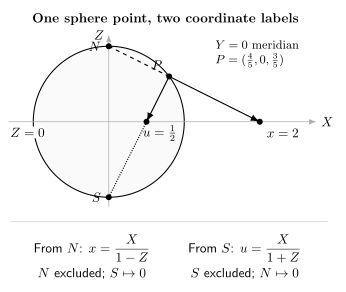
The same point $P=(4/5,0,3/5)$ on the unit sphere has north-chart coordinates $(x,y)=(2,0)$ and south-chart coordinates $(u,v)=(1/2,0)$. The straight projection lines meet $Z=0$ at different points; the transition map relates the labels, not two different sphere points. Exact $Y=0$ meridian construction.

The overlap also supplies a useful cocycle check. With only two charts, the nontrivial identities are $g_{NS}g_{SN}=\mathrm{id}$ and $g_{NN}=g_{SS}=\mathrm{id}$. For three or more charts, compatibility automatically gives $g_{\alpha\gamma}=g_{\beta\gamma}\circ g_{\alpha\beta}$ on triple overlaps. These relations are the prototype for transition-function constructions used later for bundles.

Smoothness without preferred coordinates

A function $f:M\to\mathbb R$ is smooth when $f\circ\varphi_\alpha^{-1}$ is smooth in one, and therefore every, compatible chart. More generally, $F:M\to N$ is smooth when every local representative $\psi_\beta\circ F\circ\varphi_\alpha^{-1}$ is smooth wherever defined. The chain rule and smooth transition maps prove chart independence.

This definition separates a point from its coordinate tuple. The tuples $(x,y)$ and $(u,v)$ on the stereographic overlap differ, but both label the same point of $S^2$. Any statement that depends on one tuple and fails the transition test is coordinate information, not an intrinsic property. At this stage no metric, connection, curvature, or volume has been chosen: smoothness alone permits differentiation of maps but not lengths or parallel comparison between separate tangent spaces.

Why the separation hypotheses matter

Local Euclidean appearance does not by itself guarantee acceptable global behavior. Construct the line with two origins by taking two copies of $\mathbb R$ and identifying points with the same nonzero coordinate while keeping the two origins distinct. Each origin has a neighborhood homeomorphic to an interval, and the usual coordinate transitions away from the origins are smooth. Yet any neighborhoods of the two origins intersect, so the space is not Hausdorff. A sequence of nonzero points approaching zero converges to both origins.

The example distinguishes chart compatibility from the topology needed for analysis. It does not show that every non-Hausdorff space is unusable; rather, it explains why the conventional definition deliberately excludes such spaces. Likewise, this page treats manifolds without boundary. Manifolds with boundary use charts into a half-space and require an additional boundary-compatible formulation, introduced when Stokes’ theorem is developed.

Smooth structure is also stronger than topology. A homeomorphism preserves open sets, while a diffeomorphism must preserve the chosen smooth atlases in both directions. It is therefore possible for one topological manifold to support inequivalent smooth structures. No such subtlety is needed for the standard spaces used in the calculations here, but the distinction explains why “same shape continuously” and “same smooth manifold” are different assertions. In practice, establish the topological manifold first, then specify the compatible atlas, and only afterward introduce tensors or other geometric fields.

Exercises

For the stereographic transition $F(x,y)=(x/r^2,y/r^2)$, compute its Jacobian determinant and decide whether it preserves the standard orientation of the coordinate plane.

Solution

Writing $r^2=x^2+y^2$ gives

$$DF=\frac{1}{r^4} \begin{pmatrix} y^2-x^2 & -2xy\\ -2xy & x^2-y^2 \end{pmatrix}, \qquad \det DF=-\frac{1}{r^4}.$$

The determinant is nonzero on the overlap, confirming again that the transition is a local diffeomorphism. Its negative sign means these particular coordinate orderings induce opposite orientations. Smooth compatibility does not require orientation preservation; an oriented atlas imposes that stronger condition.

References

• Gualtieri, Marco. Geometry and Topology I. University of Toronto course notes, 2017, §§1.1–1.5, pp. 2–13. Course PDF.
• Lee, John M. Introduction to Smooth Manifolds. 2nd ed., Graduate Texts in Mathematics 218, Springer, 2013, doi:10.1007/978-1-4419-9982-5.