Polarization Tests with Detector Networks

Scrollable formula. Use Left and Right arrow keys to reveal hidden content.

Scrollable table. Use Left and Right arrow keys to reveal additional columns.

Scrollable figure. Use Left and Right arrow keys to inspect hidden content.

A metric wave in a general four-dimensional theory may carry tensor, vector, or scalar polarization content, but a detector records only a projected strain. A polarization test therefore asks a rank-and-coherence question: does the network geometry contain enough independent responses to distinguish hypotheses after sky position, waveform content, calibration, noise, and selection are marginalized? Counting detectors is necessary but not sufficient; nearly aligned instruments or restrictive waveform assumptions can leave the response ill-conditioned.

Helpful background. Weak-Field Gravity defines radiative metric perturbations; Probability and Statistical Inference supplies evidence and prior comparisons; Gravitational-Wave Data Analysis and Inference supplies detector response and coherent likelihoods; Tests of Gravity supplies the operational null; and Black-Hole Perturbation Theory clarifies when source modes and polarization states are distinct objects.

Network response and identifiability

For detector $I$ and a fixed sky direction $\hat n$ , the strain is

d_I(f)=\sum_A F_I^A(\hat n,\psi,t)h_A(f)+n_I(f),

where $A\in\{+,\times,x,y,b,\ell\}$ labels two tensor, two vector, breathing-scalar, and longitudinal-scalar modes. Inter-site travel-time phases are removed using the hypothesized sky direction; otherwise they belong in $F_I^A(f)$ . The polarization angle $\psi$ specifies the transverse basis, and $F_I^A$ is the detector’s dimensionless response to a unit amplitude in that basis. In matrix form, $\mathbf d=\mathbf F\mathbf h+\mathbf n$ . Multiplying by $\mathbf N^{-1/2}$ whitens the noise: its covariance becomes the identity. Predicted signals lie in the column space of this whitened response. Polarization amplitudes differing by a vector in its kernel produce exactly the same strain. A zero singular value identifies such an invisible combination; a small singular value identifies a combination whose reconstruction greatly amplifies noise. These singular values, not the raw instrument count, determine what is measured.

In the long-wavelength limit of differential-arm interferometers, scalar breathing and longitudinal responses are linearly dependent, so they cannot be independently identified by simply adding events. For a transient with two detectors and a rank-two tensor response, two arbitrary tensor waveforms fill the data space; a tensor null stream does not exist. A rank-deficient two-detector response can have a null direction, but then loses an independent tensor measurement. Three suitably oriented detectors normally supply one null direction, while more independent responses improve conditioning. Earth rotation helps continuous signals, and a precisely localized electromagnetic counterpart removes a major sky-response degeneracy.

The scalar degeneracy follows from detector geometry. For unit arm directions $u,v$ , the long-wavelength detector tensor is $D^{ij}=(u^iu^j-v^iv^j)/2$ , whose trace is zero. With orthonormal transverse vectors $p,q$ and propagation direction $\hat n$ , choose $e^b=pp+qq$ and $e^\ell=\hat n\hat n$ . Then

F^b=D^{ij}(\delta_{ij}-\hat n_i\hat n_j) =-D^{ij}\hat n_i\hat n_j=-F^\ell.

A different longitudinal normalization changes the constant of proportionality, not the degeneracy. Finite-arm transfer functions or additional physical waveform information require a separate analysis.

A three-channel example

For equal, independent whitened noise and a fixed sky direction, consider the illustrative tensor response

F_T=\begin{pmatrix}1&0\\0&1\\1&1\end{pmatrix}, \qquad q=\frac{d_3-d_1-d_2}{\sqrt3}.

A pure tensor signal gives $(d_1,d_2,d_3)=(h_+,h_\times,h_++h_\times)$ , hence $q=0$ before noise. The normalization makes the noise variance of $q$ equal to one when each channel has unit variance. An extra response $g\,h_X$ enters the null channel with amplitude $(g_3-g_1-g_2)h_X/\sqrt3$ . If that coefficient vanishes, the extra mode lies inside the tensor response plane and this null test cannot see it. Thus even a clean null stream constrains a particular projection, not every possible extra polarization. The figure shows which part of the data survives the projection.

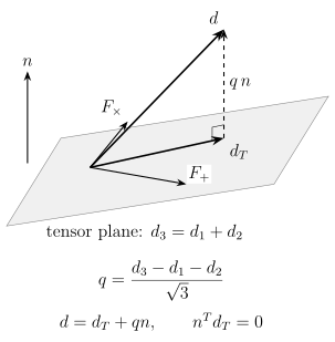
Two tensor responses span a plane in three-channel data; the perpendicular component survives in the null stream, while any extra mode inside the plane does not. — The tensor plane satisfies $d_3=d_1+d_2$ and the perpendicular unit vector is $\mathbf n=(-1,-1,1)/\sqrt3$ . The null amplitude is $q=\mathbf n\cdot\mathbf d$ . This schematic assumes a fixed sky direction, aligned arrival times, and whitened independent unit-variance noise; its toy response is not a real detector network. An extra polarization whose response lies in the plane remains invisible to this projection.

For a hypothesis with response matrix $F_H$ , a noise-weighted null projector can be written

P_H=I-F_H(F_H^\dagger N^{-1}F_H)^{-1}F_H^\dagger N^{-1}.

Under that hypothesis, $P_H\mathbf d$ should contain calibrated noise rather than coherent signal. The inverse exists only on the resolved response subspace; near-singular directions require a pseudoinverse and explicit threshold. This geometric construction is robust to some waveform uncertainty, but a model that assumes all polarizations share a fixed phase evolution may miss dipolar radiation at a different frequency.

Yunes, Siemens, and Yagi explain why null streams, pure-polarization comparisons, and mixed tensor–vector–scalar hypotheses answer different questions Yunes, Siemens, and Yagi 2025, §4.3.7, pp. 107–109. Pure scalar versus pure tensor is a useful null comparison, not necessarily a contest between two viable complete theories. A mixed-mode bound depends on the chosen basis dimension, amplitude and phase relation, source model, and prior volume.

Data, hypotheses, and covariance

To specify the likelihood normalization unambiguously, stack the real and imaginary Fourier components into one real data vector $\mathbf y$ , with real model vector $\mathbf m_H$ and covariance $C_y$ . Then

p(\mathbf y\mid H,\lambda,C) =\frac{\exp[-\tfrac12(\mathbf y-\mathbf m_H)^T C_y^{-1}(\mathbf y-\mathbf m_H)]} {(2\pi)^{n_y/2}\sqrt{\det C_y}},

where $n_y$ is the number of real components, $\lambda$ denotes waveform or wavelet parameters, and $C$ denotes calibration nuisance variables. This real-vector formula avoids mixing the determinant and factor-of-two conventions of real and complex Gaussian densities. Bayes factors compare marginal likelihoods only after priors on sky position, event time, polarization angle, relative mode amplitudes, phases, and model dimension are declared. Changing the allowed subspace changes the Occam penalty and therefore the result.

At the evidence cutoff 2026-08-19, the peer-reviewed GWTC-3 analysis gives the established catalog method: its basis choices are in Table VIII and its combined hypothesis comparisons in Tables IX–X LIGO–Virgo–KAGRA 2023, §VII and Tables VIII–X. The submitted GWTC-5 manuscript updates a null-stream implementation and identifies the tested event subsets separately LIGO–Virgo–KAGRA 2026, submitted P2500781-v17, §§2–3, §5, and Tables 1 and 5–6. Its current conclusions are conditional on an effective-polarization construction and are not a proof that only tensor modes exist in nature.

The strain and posterior inputs come from GWTC-5/GWOSC stable parameter-estimation release 9 GWOSC 2026, official parameter-estimation, strain, and data-quality documentation; P2600410-v1 separately supplies the released polarization result products LIGO–Virgo–KAGRA 2026, official tests data release. A reproducible run pins calibrated files, detector availability, quality segments, sky information, time–frequency resolution, response conventions, null-stream software, priors, sampler diagnostics, and event selection. Calibration phase covariance can imitate an inter-detector coherence error; glitches, spectral drift, and uncertain sky position can add false null energy. Completeness is hypothesis-dependent because a search optimized for tensor templates need not detect every non-tensorial signal with the same efficiency.

Results and limitations through 2026-08-19

Evidence or result	Position supported	Limitation or scope
Network antenna geometry	Three or more independent responses can form tensor-null combinations	Co-alignment, scalar degeneracy, duty cycle, and sky position can reduce effective rank
Peer-reviewed GWTC-3 catalog comparison	Selected signals were compatible with tensor polarization under the tested bases	Mixed hypotheses, waveform relations, prior volume, and O3 calibration delimit the result
Submitted GWTC-5 null-stream analysis	Current selected events strengthen several tensor-versus-nontensor comparisons	Submitted analysis; effective-mode assumptions need not represent every complete theory

The conservative position is that no resolved extra polarization has been established in these tests. A competing interpretation could invoke a weak, frequency-shifted, or source-dependent mode that the assumed basis absorbs poorly. The adversarial independent check injects tensor, scalar, vector, and mixed signals through the actual network geometry, including modes at distinct harmonics, and measures coverage and confusion as response singular values deteriorate. It must also recover noise-only null statistics from off-source data. Until such controls span the relevant theory and source population, exclusion of generic extra polarizations remains unresolved and model-dependent.

What could change the conclusion. The interpretation could change after a peer-reviewed GWTC-5 polarization result, a substantially different detector network, a released mixed-mode injection campaign, or a theory prediction that invalidates the shared-waveform basis used by present null streams.

Exercises

Why can three non-coaligned detectors form a null stream for two arbitrary tensor polarizations, and why does the same counting not separate all six nominal metric polarizations?

Solution

At a fixed frequency, two tensor amplitudes span at most a two-dimensional column space in three-detector data, so one independent linear combination is orthogonal to that space and cancels the tensor signal. Six labels do not imply six measurable directions: the response matrix has at most three rows, and breathing and longitudinal scalar responses are degenerate for long-wavelength differential-arm detectors. Therefore rank, conditioning, and waveform relations—not polarization names alone—determine what can be separated.

References

Gravitational Wave Open Science Center (2026), “GWTC-5.0 Data Release Documentation,” stable release 9 parameter-estimation, strain, and data-quality products, official release, DOI.
LIGO Scientific Collaboration, Virgo Collaboration, and KAGRA Collaboration, “Data Release for GWTC-5.0: Tests of General Relativity,” version P2600410-v1 (2026), official release.
LIGO Scientific Collaboration, Virgo Collaboration, and KAGRA Collaboration, “GWTC-5.0: Tests of General Relativity,” submitted manuscript P2500781-v17 (2026), official DCC record.
LIGO Scientific Collaboration, Virgo Collaboration, and KAGRA Collaboration, “Tests of General Relativity with GWTC-3,” Physical Review D 107, 022005 (2023), DOI.
Nicolás Yunes, Xavier Siemens, and Kent Yagi, “Gravitational-Wave Tests of General Relativity with Ground-Based Detectors and Pulsar-Timing Arrays,” Living Reviews in Relativity 28, article 3 (2025), DOI.