Lensing and Dynamical Potentials

Light deflection and slow motion do not generally measure the same metric combination. In a weakly perturbed cosmological spacetime, nonrelativistic tracers respond primarily to the time potential $\Phi$, whereas lensing responds to the Weyl combination $\Phi+\Psi$. Comparing the two can therefore test gravitational slip—but only after the source distribution, projection, distance scale, and dynamical state have been modeled consistently.

Required background. Geodesics and Jacobi Fields supplies null-ray and geodesic-deviation methods; Probability and Statistical Inference supplies normalized likelihoods and nuisance-parameter marginalization.

Helpful background. Weak-Field Gravity supplies the metric perturbation and Newtonian limits; Relativistic Cosmology supplies angular-diameter distances, growth, and light-cone projection.

Two potentials and two responses

Use conformal Newtonian gauge for scalar perturbations, written here in cosmic time $t$ with comoving spatial coordinates $\boldsymbol x$,

$$ds^2=-(1+2\Phi)dt^2+a^2(t)(1-2\Psi)d\boldsymbol{x}^2, \qquad \lvert\Phi\rvert,\lvert\Psi\rvert\ll1.$$

Here $a(t)$ is the scale factor, $H=\dot a/a$, and a dot means $d/dt$. The potentials are dimensionless in the site’s $c=1$ units; the corresponding Newtonian potential in SI units is $c^2\Phi$. For a slowly moving particle, the spatial geodesic equation gives

$$\ddot{\boldsymbol{x}}+2H\dot{\boldsymbol{x}} =-\frac{1}{a^2}\boldsymbol{\nabla}\Phi,$$

so peculiar acceleration determines gradients of $\Phi$ after expansion and tracer physics are removed. The physical peculiar velocity is $\boldsymbol v=a\dot{\boldsymbol x}$, for which $\dot{\boldsymbol v}+H\boldsymbol v=-\boldsymbol\nabla\Phi/a$. A null ray, by contrast, gives the leading angular displacement in the lens map $\boldsymbol\beta=\boldsymbol\theta-\boldsymbol\alpha(\boldsymbol\theta)$:

$$\boldsymbol{\alpha}(\boldsymbol{\theta}) =\int_0^{\chi_s}d\chi\, \frac{\chi_s-\chi}{\chi_s}\, \boldsymbol{\nabla}_{\!\perp}(\Phi+\Psi),$$

for a spatially flat background and a source at comoving distance $\chi_s$. Here $\boldsymbol\theta$ and $\boldsymbol\beta$ are image and unlensed source angles, and $\boldsymbol\nabla_\perp$ differentiates with respect to transverse comoving length, evaluated on the unperturbed ray at $\boldsymbol x_\perp=\chi\boldsymbol\theta$. This is the first-order Born approximation. Curvature changes the distance kernels, not the fact that light sees the sum. The optical tidal matrix, and hence convergence and shear, contains transverse second derivatives of that same sum.

The reduced deflection $\boldsymbol\alpha$ is different from the physical bending angle $\widehat{\boldsymbol\alpha}$ at a localized lens. In the thin-lens limit,

$$\boldsymbol\alpha=\frac{D_{ls}}{D_s}\widehat{\boldsymbol\alpha}, \qquad \widehat{\boldsymbol\alpha} =\int dz\,\boldsymbol\nabla_b(\Phi+\Psi).$$

The second integral uses local physical transverse displacement $\boldsymbol b$ and line-of-sight distance $z$; $D_l,D_s,D_{ls}$ are angular-diameter distances from observer to lens, observer to source, and lens to source. A fixed physical bend produces a smaller image–source displacement when the source lies close behind the lens. This distinction and the lens-map sign convention are developed in Bartelmann and Schneider 2001, §§3.1.1–3.1.2, Eqs. (3.1)–(3.6).

In the diagram, compare the bending angle at the lens with the separation between the image and unlensed source directions at the observer. They are connected by a distance ratio, not equality.

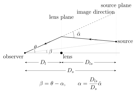
For one weak thin lens in geometric optics, the reduced deflection is $\alpha=\theta-\beta=(D_{ls}/D_s)\widehat\alpha$. Photon arrows run from source to observer; the continued line indicates the apparent image direction. Angles are exaggerated and the diagram is not to scale. In a cosmological spacetime, these angular-diameter distances need not add as Euclidean lengths.

To make the comparison explicit, define

$$-k^2\Phi=4\pi G a^2\mu(k,a)\rho_m\Delta_m, \qquad \eta_{\rm slip}(k,a)=\frac{\Psi}{\Phi},$$

and therefore

$$-k^2(\Phi+\Psi)=8\pi G a^2\Sigma(k,a)\rho_m\Delta_m, \qquad \Sigma=\frac{\mu(1+\eta_{\rm slip})}{2}.$$

Here $k$ is comoving wavenumber, $\rho_m$ is the background matter density, and $\Delta_m$ is the comoving matter-density contrast; on subhorizon scales it agrees with the usual density contrast to the accuracy of the quasistatic reduction. The spatial Fourier phase is $e^{i\boldsymbol{k}\cdot\boldsymbol{x}}$. In the linear GR limit with minimally coupled pressureless matter, a cosmological constant, and negligible other clustering or anisotropic stress, $\mu=1$, $\Phi=\Psi$, and thus $\eta_{\rm slip}=\Sigma=1$. This is a conditional null: radiation, neutrino stress, clustering additional matter, or extending the linear parameterization into nonlinear structure changes the comparison. A departure from unity must first be compared with those GR contributions.

The potentials are not raw coordinate coefficients to be compared across arbitrary gauges. In the scalar sector they may be understood as the gauge-invariant Bardeen potentials, represented here in conformal Newtonian gauge when that decomposition is valid. The actual data—angles, redshifts, arrival times, and tracer velocities—are observer-defined quantities. Deriving both predictions from those observables prevents a time-slicing change from masquerading as gravitational slip and makes the quasistatic approximation an explicit physical assumption rather than a coordinate shortcut.

From projected observables to a gravity comparison

A lensing reconstruction gives a weighted, projected field. Galaxy velocities, gas temperatures, or stellar dispersions infer a three-dimensional force only through equilibrium, anisotropy, inclination, and source assumptions. A sound comparison therefore predicts both datasets from a common latent mass distribution $\rho$:

$$p(d_{\rm lens},d_{\rm dyn}\mid\mathcal M) =\int p(d_{\rm lens}\mid\rho,\eta_L,\mathcal M) p(d_{\rm dyn}\mid\rho,\eta_D,\mathcal M) p(\rho,\eta_L,\eta_D\mid\mathcal M) \,d\rho\,d\eta_L\,d\eta_D.$$

The lens nuisances $\eta_L$ include redshift, point-spread response, shear calibration, line-of-sight structure, and mass-sheet freedom. The dynamical nuisances $\eta_D$ include tracer selection, velocity anisotropy, pressure support, mass-to-light ratio, and nonequilibrium. Shared distance, center, ellipticity, and environment parameters require covariance; fitting the two sides separately and dividing their reported masses discards it.

The result is also scale and environment dependent. The quasistatic, subhorizon reduction can fail near horizon scales or for rapidly evolving extra fields. Screening can restore $\mu\simeq\eta_{\rm slip}\simeq1$ in a dense lens while leaving cosmological growth modified. Converting a projected lens mass to a spherical dynamical mass can manufacture apparent slip when the lens is triaxial or embedded in correlated structure. A reconstructed mass map is therefore not a direct metric measurement.

Checks and limitations

For a static spherical point mass, $\Phi=\Psi=-GM/r$. Along an unperturbed ray with impact parameter $b$, $r^2=b^2+z^2$, so

$$\widehat\alpha =2GMb\int_{-\infty}^{\infty}\frac{dz}{(b^2+z^2)^{3/2}} =\frac{4GM}{b}, \qquad \alpha=\frac{D_{ls}}{D_s}\frac{4GM}{b}.$$

Slow circular motion gives $v_c^2=GM/r$. Evaluating it at $r=b$ yields $\alpha=4(D_{ls}/D_s)v_c^2$; restoring SI units replaces $v_c^2$ by $v_c^2/c^2$. This checks both the factor of two in relativistic light bending and the source-distance factor. A second check is conformal: multiplying the metric by $1+2\epsilon$ shifts $\Phi\to\Phi+\epsilon$ and $\Psi\to\Psi-\epsilon$ at this order. Their sum, and hence unparameterized null paths, stays unchanged.

Neither check removes source degeneracy. Dark matter under GR, modified field equations with baryons alone, and a biased dynamical tracer may predict similar projected comparisons. One should also compare the joint model with lens-only and dynamics-only posterior predictive distributions: an apparent slip that is driven by one poorly fitted tracer is not evidence that the two metric potentials differ. Splitting the sample by morphology and environment tests whether a universal parameter is hiding object-dependent source errors. The physical conclusion is bounded: a joint analysis constrains the declared $\mu$–$\eta_{\rm slip}$ parameterization over its redshift, wavenumber, morphology, and screening domain; it does not identify a unique action.

Exercise

A spherical lens has $\Phi=-GM/r$ but $\Psi=\gamma\Phi$, with constant $\gamma$ over the ray. Find the physical and reduced deflection magnitudes and compare them with the circular speed at radius $r$.

Solution

The transverse gradient of $\Phi+\Psi=-(1+\gamma)GM/r$ integrates along the unperturbed line of sight to $\widehat\alpha=2(1+\gamma)GM/b$. The angular displacement is $\alpha=(D_{ls}/D_s)\widehat\alpha$. Slow orbital motion still responds to $\Phi$, so $v_c^2=r\,d\Phi/dr=GM/r$. At $r=b$, $\alpha/[4(D_{ls}/D_s)v_c^2]=(1+\gamma)/2$. Thus the geometrically matched lensing-to-dynamics ratio measures $(1+\gamma)/2$ relative to its GR value. Allowing independent source normalizations or omitting the distance factor would absorb or imitate the slip signal.

References

• Bartelmann, M., and Schneider, P. (2001), “Weak Gravitational Lensing,” Physics Reports 340, 291–472. DOI.

Further reading

• Ferreira, P. G. (2019), “Cosmological Tests of Gravity,” Annual Review of Astronomy and Astrophysics 57, 335–374. DOI.
• Ishak, M. (2019), “Testing General Relativity in Cosmology,” Living Reviews in Relativity 22, article 1. DOI.