Parameterized Post-Keplerian Timing

Parameterized post-Keplerian (PPK) timing separates what a relativistic binary’s pulse arrival times measure from what a particular gravity theory predicts. Keplerian parameters describe the leading orbit; post-Keplerian parameters describe relativistic timing effects without initially imposing a mass relation. A theory is tested only when it maps the component masses and any additional charges to several independently measured post-Keplerian quantities.

Required background. Weak Metric Perturbations and Gauge Freedom supplies weak-field gravity and post-Newtonian ordering. Probability and Inference for Gravity supplies likelihood, covariance, and joint parameter inference.

Helpful background. Relativistic Two-Body Dynamics supplies conservative orbital dynamics, radiation reaction, and mass combinations used in timing predictions.

From pulse phase to a relativistic orbit

A timing model predicts the barycentric arrival time of each pulse from the pulsar’s rotation, astrometry, interstellar propagation, Solar-System ephemeris, and binary motion. The Keplerian sector includes orbital period $P_b$, eccentricity $e$, projected semimajor axis $x=a_p\sin i$, longitude of periastron $\omega$, and an orbital epoch. Relativistic corrections are then represented by phenomenological post-Keplerian parameters.

Common examples are periastron advance $\dot\omega$, the combined gravitational-redshift and second-order Doppler amplitude $\gamma_E$, Shapiro range $r$ and shape $s$, and orbital-period derivative $\dot P_b$. The subscript on $\gamma_E$ distinguishes this timing amplitude from the PPN parameter $\gamma$. Other useful quantities include changes in projected semimajor axis, orbital deformation parameters, and spin-precession observables.

The key separation is

$$\text{arrival-time data} \longrightarrow \{P_b,e,x,\dot\omega,\gamma_E,r,s,\dot P_b,\ldots\} \longrightarrow \text{theory test}.$$

The first arrow is a fit to a timing model with correlated noise and propagation terms. The second inserts theory-specific relations among masses, charges, and timing parameters.

Overdetermination in general relativity

For nonspinning point masses $m_p$ and $m_c$ with $M=m_p+m_c$, GR predicts at leading post-Newtonian order

$$\dot\omega =\frac{3}{1-e^2} \left(\frac{2\pi}{P_b}\right)^{5/3}(GM)^{2/3},$$

and, for the Einstein-delay amplitude,

$$\gamma_E =e\left(\frac{P_b}{2\pi}\right)^{1/3} G^{2/3}\frac{m_c(m_p+2m_c)}{M^{4/3}}.$$

At leading order the Shapiro parameters are $r=Gm_c$ and $s=\sin i$. The quadrupolar orbital-decay prediction can be written

$$\dot P_b^{\rm GR} =-\frac{192\pi}{5} \left(\frac{2\pi G\mathcal M}{P_b}\right)^{5/3} \frac{1+73e^2/24+37e^4/96}{(1-e^2)^{7/2}},$$

where $\mathcal M=(m_pm_c)^{3/5}M^{-1/5}$ is the chirp mass. These formulae use $c=1$ and omit higher-order, spin, and finite-size terms when those are below the required accuracy.

Two post-Keplerian measurements can determine $m_p$ and $m_c$ under GR. Every additional measurement then draws another curve in the mass plane; consistency requires the curves to intersect within their joint uncertainty. This overdetermination is more informative than fitting a separate mass pair for each effect. Freire and Wex develop the timing observables and their theory mappings in detail Freire and Wex 2024, §3.4.2, Eqs. (28)–(34), §3.5.1, Eq. (35).

A synthetic three-quantity test

Take $m_p=1.4M_\odot$, $m_c=1.2M_\odot$, $P_b=0.3$ day, and $e=0.2$. These are illustrative inputs, not a measured system. To evaluate the equations in seconds with masses expressed in solar units, use $T_\odot=GM_\odot/c^3=4.925490947\,\mu\mathrm s$ as the declared conversion. The leading-order predictions are

$$\dot\omega\simeq2.91474\;\mathrm{deg\,yr^{-1}},\qquad \gamma_E\simeq1.18435\;\mathrm{ms},\qquad r\simeq5.91059\;\mu\mathrm s,$$

where a year is 365.25 days. Inverting $r$ fixes $m_c$; inverting $\dot\omega$ fixes $M$. Their intersection therefore determines $m_p=M-m_c$. The third quantity $\gamma_E$ is now predicted. Inspect the figure’s common point: shifting only the third input by 10% makes its curve miss that point even though each individual curve still permits many masses.

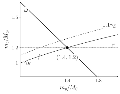
Synthetic leading-PN GR curves for the specified 0.3-day, eccentricity-0.2 binary. The total-mass constraint from $\dot\omega$ and the companion-mass constraint from Shapiro range $r$ meet at $(1.4,1.2)M_\odot$. The Einstein-delay curve passes through that point; a dashed curve for a 10% larger delay does not. There are no observational data or uncertainty bands, and the shifted input is a consistency diagnostic rather than a complete alternative theory.

The plot intentionally omits measurement errors to isolate the logic. An actual analysis uses correlated likelihood regions, verifies that each timing quantity is identifiable for the observed inclination and cadence, and includes higher-order corrections when the precision requires them. A visually narrow intersection alone is not a calibrated goodness-of-fit test.

Kinematic and environmental corrections

The observed period derivative is not yet the intrinsic binary decay:

$$\dot P_b^{\rm rad} =\dot P_b^{\rm obs} -\dot P_b^{\rm Shk} -\dot P_b^{\rm Gal} -\dot P_b^{\rm mass,loss} -\cdots.$$

Here the target is the radiative contribution, so the right-hand side also removes intrinsic nonradiative processes such as mass loss. In a convention where “intrinsic” means only kinematically corrected, mass loss remains in $\dot P_b^{\rm int}$ and must be included in its predicted model instead. The Shklovskii term arises from transverse motion and depends on proper motion and distance. Differential acceleration between the binary and Solar System in the Galactic potential contributes another correction. Tides, cluster acceleration, and line-of-sight companions may matter in particular systems. These corrections carry shared astrometric and Galactic-model uncertainty and must enter the likelihood rather than being subtracted as exact numbers Kramer et al. 2021, §V, §VI.B.1–5, and Eqs. (39)–(48).

Timing noise, dispersion-measure variation, pulse-profile evolution, clock standards, and the Solar-System ephemeris can correlate with orbital parameters. Dataset spans, radio-frequency coverage, backend offsets, noise model, and software version are therefore parts of the test even though the PPK definitions themselves are stable.

Theory-agnostic does not mean theory-free

The fitted PPK parameters are phenomenological, but their interpretation always invokes a theory. A scalar-tensor model, for example, can introduce body sensitivities, scalar charges, and dipole radiation. The conservative parameters and $\dot P_b$ then depend on the equation of state and cosmological scalar boundary value as well as the masses. One cannot obtain the theory constraint by changing only the quadrupole formula while leaving the conservative mass solution fixed to GR.

The PPK framework is strongest when several effects have distinct mass and inclination dependence. It becomes weak when parameters are highly covariant, the data span is too short, or an external distance dominates $\dot P_b^{\rm int}$. A complete result reports the joint timing covariance and tests alternative red-noise, dispersion, and ephemeris models.

Check your understanding

Why do three accurately measured post-Keplerian parameters test GR, whereas two usually determine masses under GR? Explain what happens if the third curve misses the common intersection.

Solution

GR maps each post-Keplerian parameter, together with the measured Keplerian orbit, to a curve in the two-dimensional $(m_p,m_c)$ plane. Two nondegenerate curves therefore determine a mass pair. The third parameter is then predicted rather than freely fitted at the theory level, so its curve must pass through the same uncertainty region. If it misses, the composite model is inconsistent. One must first check timing noise, kinematic corrections, finite-size or spin terms, and joint covariance; only after those alternatives fail does the discrepancy motivate a different gravitational mapping.

References

• Freire, P. C. C., and Wex, N. (2024), “Gravity experiments with radio pulsars,” Living Reviews in Relativity 27, 5. Freire and Wex 2024, §§3.4–3.5 and §§4–5.
• Kramer, M., et al. (2021), “Strong-field gravity tests with the double pulsar,” Physical Review X 11, 041050. Kramer et al. 2021, §§III–VI and Table IV.