Vainshtein Screening

Vainshtein screening suppresses a scalar force by making second-derivative self-interactions dominate near a source. The scalar field itself need not be small: its radial gradient becomes small relative to the linear solution. The mechanism is therefore a nonlinear branch-matching problem, not a large mass or weak coupling. This page fixes one cubic-Galileon normalization, derives its Vainshtein radius, and states the environment and cutoff conditions under which “recovery of GR” is meaningful.

Required background. Ordinary Differential Equations supplies the radial first integral and asymptotic matching used below.

Helpful background. Einstein Equations supplies the GR comparison force; Gravitational Actions and Boundary Terms supplies variational signs and surface terms; Formulations of General Relativity supplies branch and constraint language; Gravity Beyond General Relativity supplies mode and cutoff checks; and Relativistic Matter and Compact Objects supplies the strong-field sources for which this decoupling calculation is not sufficient.

Cubic derivative interaction

Use the reduced Planck mass $M_{\rm Pl}^{-2}=8\pi G$, take $\Lambda\gt0$, $\beta\gt0$, and a positive source mass, and consider

$$S_\pi=\int d^4x\left[ -\frac12(\partial\pi)^2 -\frac{1}{2\Lambda^3}(\partial\pi)^2\Box\pi +\frac{\beta}{M_{\rm Pl}}\pi T \right].$$

Although the Lagrangian contains second derivatives, its Euler–Lagrange equation contains no derivative higher than second order:

$$\Box\pi+\frac{1}{\Lambda^3} \left[(\Box\pi)^2 -(\partial_\mu\partial_\nu\pi) (\partial^\mu\partial^\nu\pi)\right] =-\frac{\beta T}{M_{\rm Pl}}.$$

For nonrelativistic matter $T\simeq-\rho$. The relative minus sign between the two quadratic Hessian contractions is what removes third derivatives. The cubic Galileon and its Vainshtein limit are developed in Joyce et al. 2015, §§ 6.2.1–6.2.3.

We work on the asymptotically decaying, static spherical branch outside a source of radius $R$, with $r\geq R$, while metric backreaction and time derivatives are negligible. These assumptions define the calculation; they do not follow merely from $r\lt r_V$.

First integral and Vainshtein radius

For $\pi=\pi(r)$, the equation becomes a total radial derivative:

$$\frac{1}{r^2}\frac{d}{dr} \left[r^2\pi' +\frac{2}{\Lambda^3}r(\pi')^2\right] =\frac{\beta\rho}{M_{\rm Pl}}.$$

Outside the source, integration over the enclosed mass gives

$$r^2\pi'+\frac{2}{\Lambda^3}r(\pi')^2=C, \qquad C\equiv\frac{\beta M}{4\pi M_{\rm Pl}}.$$

Define, in this normalization,

$$r_V^3\equiv\frac{8C}{\Lambda^3} =\frac{2\beta M}{\pi M_{\rm Pl}\Lambda^3}.$$

The branch that approaches zero gradient at infinity is

$$\boxed{ \pi'(r)=\frac{\Lambda^3r}{4} \left[ -1+\sqrt{1+\left(\frac{r_V}{r}\right)^3} \right] }.$$

Substitution into the quadratic first integral independently checks every coefficient. Dimensional analysis also works: $r_V^3$ has mass dimension $-3$, while $\pi'$ has dimension two. The opposite square-root branch grows as $-\Lambda^3r/2$ at large radius and is not the asymptotically decaying solution selected here.

Far and screened zones

For $r\gg r_V$, expand the square root:

$$\pi'=\frac{C}{r^2} \left[1+O\!\left((r_V/r)^3\right)\right].$$

The scalar acceleration of an unscreened test body is $a_\pi=\beta\pi'/M_{\rm Pl}$. Hence

$$\frac{a_\pi}{a_N}\longrightarrow 2\beta^2, \qquad r\gg r_V.$$

For $R\ll r\ll r_V$,

$$\pi'\simeq \frac{\Lambda^3}{4}r_V^{3/2}r^{-1/2}, \qquad \boxed{ \frac{a_\pi}{a_N}\simeq 4\beta^2\left(\frac{r}{r_V}\right)^{3/2} }.$$

The absolute gradient grows toward the source as $r^{-1/2}$, but the Newtonian force grows faster, as $r^{-2}$. “Screened” refers to their ratio. At $r\sim r_V$, neither asymptotic series is reliable; the exact branch supplies the matching.

The matching is particularly transparent in dimensionless form:

$$x=\frac{r}{r_V}, \qquad \frac{a_\pi}{2\beta^2a_N} =\frac{2}{1+\sqrt{1+x^{-3}}}.$$

This rationalized expression is also numerically stable at large $x$, where subtracting one from the square root in $\pi'$ would lose precision. It rises monotonically from $2x^{3/2}$ to one. The radius $r_V$ is a normalization of the crossover scale, not a surface separating two exact solutions.

The figure shows the exact ratio and both asymptotes. The marked point $x=1/2$ is where the linear and quadratic terms of the first integral are equal; the exact force there is half its unscreened value.

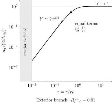
Exact exterior force ratio $Y=a_\pi/(2\beta^2a_N)$ against $x=r/r_V$ for the decaying cubic branch. The dashed inner asymptote is $Y=2x^{3/2}$; the dotted horizontal line is the unscreened limit $Y=1$. The illustrative source radius is $R/r_V=0.01$; its interior is excluded. This quantitative profile assumes a static spherical source, weak gravity, and the stated decoupling equation. It does not establish that the effective theory remains valid at every plotted radius.

Fluctuations and the effective coupling

Write $\pi=\bar\pi(r)+\varphi$. The quadratic fluctuation action has the form

$$S_\varphi^{(2)} =-\frac12\int d^4x\, Z^{\mu\nu}(\bar\pi) \partial_\mu\varphi\partial_\nu\varphi +\frac{\beta}{M_{\rm Pl}}\int d^4x\,\varphi\,\delta T.$$

Inside $r_V$, the correctly signed temporal and spatial coefficients of $Z^{\mu\nu}$ can become large. Canonical normalization therefore reduces the coupling of fluctuations to matter. Because $Z^{\mu\nu}$ is Lorentzian, health does not mean that all four coordinate eigenvalues are positive: the time-kinetic sign, spatial gradient form, and characteristic cone must be checked on the chosen background.

For the decaying cubic branch derived above, those coefficients can be checked directly. With $Z^{0i}=0$, write the principal quadratic action as

$$S_{\varphi,\mathrm{principal}}^{(2)} =\frac12\int d^4x\left[ K_t\dot\varphi^2-K_r(\partial_r\varphi)^2 -\frac{K_\Omega}{r^2}(\nabla_\Omega\varphi)^2 \right],$$

where

$$\begin{aligned} K_t&=1+\frac{2}{\Lambda^3} \left(\bar\pi''+\frac{2\bar\pi'}r\right),\\ K_r&=1+\frac{4\bar\pi'}{\Lambda^3r},\\ K_\Omega&=1+\frac{2}{\Lambda^3} \left(\bar\pi''+\frac{\bar\pi'}r\right). \end{aligned}$$

Using the screened asymptotic profile gives

$$(K_t,K_r,K_\Omega)\simeq \left(\frac34,1,\frac14\right) \left(\frac{r_V}{r}\right)^{3/2},$$

so all three coefficients have the healthy short-wavelength signs on this branch, but

$$c_r^2=\frac{K_r}{K_t}\longrightarrow\frac43, \qquad c_\Omega^2=\frac{K_\Omega}{K_t}\longrightarrow\frac13.$$

The radial scalar characteristic is therefore wider than the minimally coupled matter cone in this decoupling calculation, whereas angular propagation is subluminal. This does not by itself construct a closed causal curve, but it proves that suppression of the static fifth force is not the same statement as recovery of the matter light cone. The stability and characteristic analysis for Galileon spherical backgrounds is developed in Nicolis, Rattazzi, and Trincherini 2009, § 1.5, Eqs. (61)–(76). Other branches or environments can instead develop a wrong kinetic sign, gradient instability, or loss of hyperbolicity.

Regime and cutoff checks

The classical nonlinear balance uses $\partial^2\bar\pi/\Lambda^3\gtrsim1$. That does not by itself invalidate the derivative EFT, because operators are organized by both fields and derivatives and Galileon interactions have a special nonrenormalization structure. Nevertheless, the result is controlled only if omitted operators, metric mixing, source size, time dependence, and the local fluctuation strong-coupling scale are all quantified. Joyce et al. emphasize this EFT interpretation in Joyce et al. 2015, §§ 6.2.1–6.2.3.

Environment matters as well. Multiple sources do not generally superpose; $r_V$ is not a material surface; and a cosmological time-dependent background changes both the branch and $Z^{\mu\nu}$. The calculation above establishes a controlled decoupling-limit force ratio for one isolated spherical branch. It does not establish that a full relativistic solution is exactly GR inside the Vainshtein region.

Common pitfalls

The scalar is small inside the Vainshtein radius. Its gradient can be large. What becomes small is its force relative to the linear extrapolation or to the Newtonian force.

Large nonlinearities prove strong coupling. Classical nonlinearity and quantum loss of control are separate comparisons. The latter requires the fluctuation normalization and all omitted operators on the actual background.

Exercise

Starting from the first integral, recover the near-zone power law and find the radius at which the linear and quadratic terms have equal magnitude. Explain why this is also an independent normalization check on $r_V$.

Solution

In the nonlinear zone, drop $r^2\pi'$ and solve $2r(\pi')^2/\Lambda^3=C$. This gives $\pi'=\sqrt{C\Lambda^3/(2r)}\propto r^{-1/2}$. Equating the two terms gives $r^2\pi'=2r(\pi')^2/\Lambda^3$, or $\pi'=\Lambda^3r/2$. Substitution back into the full first integral yields $C=\Lambda^3r^3$ exactly at equal contribution. Using the exact-solution definition $r_V^3=8C/\Lambda^3$, the two terms become equal at $r=r_V/2$. At that radius the normalized force ratio is $1/2$. This comparison is physically exterior only if $R\lt r_V/2$. The exact numerical definition was chosen so that the square root is $\sqrt{1+(r_V/r)^3}$; physical screening scalings do not depend on that naming convention.

References

• Joyce, Austin, Bhuvnesh Jain, Justin Khoury, and Mark Trodden (2015), “Beyond the Cosmological Standard Model,” Physics Reports 568, 1–98. DOI. Open PDF.
• Nicolis, Alberto, Riccardo Rattazzi, and Enrico Trincherini (2009), “The Galileon as a Local Modification of Gravity,” Physical Review D 79, 064036. DOI. Open PDF.