Debris Energy Spread and Fallback

Fallback is the rate at which bound stellar debris returns to pericenter, not automatically the accretion rate and still less automatically a luminosity in one band. Its canonical $t^{-5/3}$ tail follows from a specific chain: a frozen debris-energy distribution, Keplerian return, and a finite nonzero $dM/d\varepsilon$ near zero binding energy. This page derives that chain, shows exactly how it fails, and states what a light-curve comparison must add. Generic stellar dynamics and exact geodesic derivations are outside scope.

Required background. Geodesics and Jacobi Fields supplies orbital energy and return-time concepts used in the debris mapping.

Helpful background. Black-Hole Geometry and Mechanics supplies the capture boundary; Relativistic Matter and Compact Objects supplies stellar structure and hydrodynamics; and Black-Hole Astrophysics supplies accretion and transient inference.

Freeze-in creates an energy distribution

Use the specific orbital energy $\varepsilon$, with $\varepsilon=0$ for the stellar center of mass on a Newtonian parabolic orbit and $\varepsilon<0$ for bound debris. In the impulsive approximation, the black-hole potential varies across the star at the tidal radius $r_t$, producing the characteristic spread

$$\Delta\varepsilon \simeq\frac{GM_{\rm BH}R_*}{r_t^2}.$$

Replacing $r_t$ by pericenter introduces a $\beta^2$ dependence, where $\beta=r_t/r_p$. That replacement is not justified within a model in which debris energies have already frozen near $r_t$: freely falling elements conserve their orbital energies even while their instantaneous potential energies change. Hydrodynamic and relativistic effects can alter the freeze-in picture, so weak dependence on $\beta$ is an approximation for suitable full disruptions, not a theorem for every encounter.

A uniform distribution is the simplest model,

$$\frac{dM}{d\varepsilon} \simeq\frac{M_*}{2\Delta\varepsilon}, \qquad -\Delta\varepsilon<\varepsilon<\Delta\varepsilon.$$

It is not a statement that a star has uniform density. Slicing a spherical star along the black-hole direction maps its density profile into $dM/d\varepsilon$; central concentration controls the rise and peak. Rossi and collaborators give the impulsive derivation and the density-profile integral explicitly (Rossi et al. 2021, §2.2, Eqs. 21–27).

To see the mapping, let $x$ measure position through the stellar center along the tidal direction and choose its sign so that $\varepsilon=\Delta\varepsilon\,x/R_*$. A thin slice has

$$\frac{dM}{dx}=2\pi\int_{\lvert x\rvert}^{R_*}\rho(s)s\,ds, \qquad \frac{dM}{d\varepsilon}=\frac{R_*}{\Delta\varepsilon}\frac{dM}{dx}.$$

Here $\rho(s)$ is the initial spherical density profile. Even a uniform-density sphere gives a curved distribution, $dM/d\varepsilon=3M_*[1-(\varepsilon/\Delta\varepsilon)^2]/(4\Delta\varepsilon)$, because slices near its poles have less area. The often-used flat distribution simplifies the energy distribution, not the stellar density.

The return-time Jacobian

A bound Kepler orbit with specific energy $\varepsilon=-GM_{\rm BH}/(2a)$ has return time

$$t(\varepsilon) =\frac{2\pi GM_{\rm BH}} {\left(2\lvert\varepsilon\rvert\right)^{3/2}}.$$

Inverting and differentiating gives

$$\lvert\varepsilon(t)\rvert =\frac{1}{2} \left(\frac{2\pi GM_{\rm BH}}{t}\right)^{2/3}, \qquad \left\lvert\frac{d\varepsilon}{dt}\right\rvert =\frac{1}{3}(2\pi GM_{\rm BH})^{2/3}t^{-5/3}.$$

Mass conservation then supplies the central result,

$$\dot M_{\rm fb}(t) =\left.\frac{dM}{d\varepsilon}\right|_{\varepsilon(t)} \left\lvert\frac{d\varepsilon}{dt}\right\rvert .$$

For constant $dM/d\varepsilon$, the most-bound return time and fallback rate are

$$t_{\min} =\frac{\pi}{\sqrt{2}} \left(\frac{R_*^3}{GM_*}\right)^{1/2} \left(\frac{M_{\rm BH}}{M_*}\right)^{1/2}, \qquad \dot M_{\rm fb} =\frac{M_*}{3t_{\min}} \left(\frac{t}{t_{\min}}\right)^{-5/3}.$$

Dimensions provide an immediate check: $t_{\min}$ is a stellar dynamical time multiplied by the square root of the mass ratio, while $M_*/t_{\min}$ is a rate. Integrating the idealized bound-side curve from $t_{\min}$ to infinity returns $M_*/2$, the assumed bound half of a parabolic disruption.

For $M_{\rm BH}=10^6M_\odot$, $M_*=M_\odot$, and $R_*=R_\odot$, this gives $t_{\min}\simeq41$ days and an initial flat-distribution rate of about $3.0M_\odot\,{\rm yr}^{-1}$. This is a teaching model: a smooth stellar density profile gives zero mass density at the extreme energy endpoint and hence a gradual rise rather than an abrupt turn-on at this rate. The clock starts at disruption, not at discovery or at optical maximum.

The figure compares that flat-energy model with the uniform-density sphere derived above. In the latter case,

$$\dot M_{\rm fb}(t)=\frac{M_*}{2t_{\min}} \left[1-\left(\frac{t}{t_{\min}}\right)^{-4/3}\right] \left(\frac{t}{t_{\min}}\right)^{-5/3},\qquad t\geq t_{\min}.$$

Notice the zero rate at first return and the later peak; neither feature changes the limiting exponent. Both curves integrate to the same bound mass.

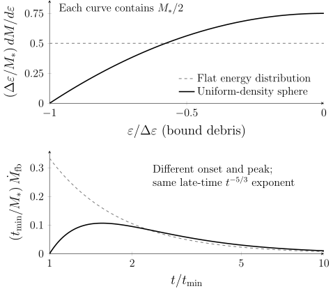
The energy distribution determines the rise as well as the late fallback. Dashed curves assume flat $dM/d\varepsilon$; solid curves use the spherical slicing result for constant stellar density. Each model returns $M_*/2$. These are quantitative Newtonian impulse models with time measured from disruption, not predicted light curves; a constant-density star is an illustrative density profile, not a realistic stellar model.

When the canonical tail changes

Suppose the distribution near zero energy behaves as

$$\frac{dM}{d\varepsilon}\propto \lvert\varepsilon\rvert^\alpha.$$

Because $\lvert\varepsilon\rvert\propto t^{-2/3}$, the late-time slope becomes

$$\dot M_{\rm fb}\propto t^{-(5+2\alpha)/3}.$$

For a power law extending all the way to zero energy, finite mass requires $\alpha\gt-1$. The $-5/3$ index requires $\alpha=0$ within the frozen, Keplerian mapping; it is not a universal definition of a tidal event. A surviving core can keep exchanging energy with marginally bound debris, in which case a time-independent $dM/d\varepsilon$ need not exist. Evolved stars, eccentric center-of-mass orbits, self-gravity, shocks, stellar spin, and relativistic energy shifts can also change the peak or tail.

Guillochon and Ramirez-Ruiz evolved 43 Newtonian FLASH 4.0 hydrodynamic encounters for $M_{\rm BH}=10^6M_\odot$, $M_*=M_\odot$, polytropes with $\gamma=4/3$ or $5/3$, and penetration factors spanning no mass loss through deep disruption. Their published grid finds partial-disruption tails approaching indices near $-2.2$ and transient slopes as steep as $-4$, whereas full disruptions approach the flat-center $-5/3$ limit (Guillochon & Ramirez-Ruiz 2013, §§2.1–2.2 and 3.2, Eq. 1, Fig. 7, and Appendix A). These numbers are benchmarks for that stellar model, gravity, resolution, and core-selection rule—not calibration constants for every star.

From fallback to a measured light curve

As of the 2026-08-18 evidence cutoff, use the named 43-run simulation grid above as a model dataset, not as an observed transient sample. It states code version, equation of state, $\beta$ selection, AMR strategy, energy convention, and cell criteria. The published article and fit coefficients are available, but a versioned public archive of every raw FLASH field is not identified; exact raw-data reproduction is therefore outside the available data product. A defensible reproduction can recover the analytic Jacobian, digitize only with an explicit added uncertainty, or rerun a separately documented model without claiming bitwise identity.

For an observed event, the source-frame fallback must pass through a delay and emission model before comparison with detector-frame data:

$$F_b(t_{\rm obs})= \frac{1}{4\pi D_L^2} \int K_b(t_{\rm src}-t')\, \eta(t')\dot M_{\rm fb}(t')\,dt' +F_{b,\rm host}, \qquad t_{\rm obs}=(1+z)t_{\rm src}.$$

Here $F_b$ is a calibrated band-integrated energy flux and $\eta\dot M_{\rm fb}$ is a power in $c=1$ units; restoring $c$ gives $\eta\dot M_{\rm fb}c^2$. The causal kernel vanishes for negative delays and has units of inverse source-frame time. Its integral specifies the fraction emerging in band $b$, including redshift-dependent spectral and bandpass corrections. A kernel depending only on $t_{\rm src}-t'$ assumes a linear, time-independent response; an evolving photosphere generally requires $K_b(t_{\rm src},t')$ or a nonlinear radiation model. Instrument counts require a further spectral response calculation, not just division by $4\pi D_L^2$. Calibration must specify photometric zero points, host subtraction, Galactic and host extinction, time system, distance, and bolometric correction. Selection must record trigger threshold, cadence, seasonal gaps, nuclear offset, classification cuts, upper limits, and whether the rise and peak were observed.

A likelihood may compare multi-band detections and censored upper limits while sampling priors on $M_{\rm BH}$, $M_*$, stellar structure, $\beta$, disruption time, delay, extinction, and reprocessing. Statistical credible intervals conditional on that model must be separated from systematic shifts between fallback-tracing and reprocessing hypotheses. Observed post-peak optical declines can resemble $t^{-5/3}$ even though rise times, temperatures, and X-ray evolution do not follow the simplest fallback prediction (Gezari 2021, §§3.1–3.2, 4.2–4.3 and Fig. 9).

Inference diagnostic

Near zero energy, a simulation yields $dM/d\varepsilon\propto\lvert\varepsilon\rvert^{1/2}$. Its synthetic optical light curve nevertheless declines as $t^{-5/3}$ after convolution with an adjustable reprocessing kernel. What is the true fallback index, and may the optical slope be used to select the flat-energy model?

Solution

Setting $\alpha=1/2$ in the Jacobian result gives

$$\dot M_{\rm fb}\propto t^{-(5+2\alpha)/3}=t^{-2}.$$

The fallback is therefore steeper than $t^{-5/3}$. The optical slope cannot select $\alpha=0$ because the fitted kernel has enough freedom to map a $t^{-2}$ input into the same band-limited decline. One must compare posterior predictions for the rise, temperature, bolometric luminosity, spectra, X-rays, and late-time behavior under both kernels, using the actual cadence and upper limits. The diagnostic separates an orbital Jacobian from a model-dependent radiation layer.

References

• Gezari, S. “Tidal Disruption Events.” Annual Review of Astronomy and Astrophysics 59, 21–58 (2021). DOI.
• Guillochon, J., & Ramirez-Ruiz, E. “Hydrodynamical Simulations to Determine the Feeding Rate of Black Holes by the Tidal Disruption of Stars: The Importance of the Impact Parameter and Stellar Structure.” The Astrophysical Journal 767, 25 (2013). DOI.
• Rossi, E. M., Stone, N. C., Law-Smith, J. A. P., et al. “The Process of Stellar Tidal Disruption by Supermassive Black Holes: The First Pericenter Passage.” Space Science Reviews 217, 40 (2021). DOI.