Mode Coupling and Nonlinear Resonance

Nonlinear field equations mix modes. At quadratic order, two oscillations drive sum and difference frequencies; angular momentum and parity decide which daughter harmonics are allowed. Resonant enhancement requires a suitable frequency match and sufficient coherence time, while damping limits the accumulated response. A peak at a combination frequency is therefore evidence of coupling, not automatically evidence of a long-lived resonance.

Helpful background. Black-Hole Geometry and Mechanics supplies background symmetries; Black-Hole Perturbation Theory supplies linear modes and damping; Formulations of General Relativity supplies nonlinear expansion; Relativistic Two-Body Dynamics supplies driving frequencies; Computational Relativity supplies spectral diagnostics.

Quadratic forcing

Expand a field or metric observable as

$$\Psi=\varepsilon\Psi^{(1)} +\varepsilon^2\Psi^{(2)}+\cdots .$$

The equations take the schematic form

$$L\Psi^{(1)}=0, \qquad L\Psi^{(2)}=S^{(2)}[\Psi^{(1)},\Psi^{(1)}].$$

If two parent modes behave as

$$\Psi_j^{(1)}=A_jY_{\ell_jm_j}e^{-i\omega_jt}, \qquad \Psi_k^{(1)}=A_kY_{\ell_km_k}e^{-i\omega_kt},$$

their products drive sum and difference frequencies and their complex-conjugate partners. If $\omega_j$ and $\omega_k$ are real, these are $\omega_j+\omega_k$ and $\omega_j-\omega_k$. For damped modes with complex frequencies, the product with the conjugate parent instead has frequency $\omega_j-\bar\omega_k$: its damping rates add rather than subtract. The azimuthal rule is

$$m_i=m_j+m_k$$

for the sum channel. Angular Clebsch–Gordan coupling requires

$$|\ell_j-\ell_k|\le\ell_i\le\ell_j+\ell_k, \qquad \ell_i+\ell_j+\ell_k \ \text{compatible with parity}.$$

Spin-weighted harmonics obey the analogous rules with spin weight included. These conditions say a coupling coefficient can be nonzero; they do not say it is large.

Second-order black-hole perturbation calculations explicitly produce quadratic source terms and radiation at combination frequencies Gleiser et al. 1996, Eqs. (1)–(18), pp. L117–L124 and Ioka and Nakano 2007, Eqs. (1)–(12), pp. 1–5.

Resonant amplitude equation

Write the daughter’s linear time dependence as $e^{-i\omega_i t-\gamma_i t}$, now using real $\omega_i$ and positive damping rate $\gamma_i$. Factor out $e^{-i\omega_i t}$ and project onto the daughter. This gives the illustrative amplitude equation

$$\dot A_i+\gamma_iA_i =C_{ijk}A_jA_k e^{-i\Delta\omega t}, \qquad \Delta\omega=\omega_j+\omega_k-\omega_i.$$

Here the parent frequencies in $\Delta\omega$ are also real; their damping or varying envelopes belong in $A_j(t)A_k(t)$. This is a reduced model, not a claim that quasinormal modes form an ordinary orthogonal basis. For constant parents set $F=C_{ijk}A_jA_k$ and take $A_i(0)=0$. Multiplication by the integrating factor $e^{\gamma_i t}$ gives

$$A_i(t) =F\,\frac{e^{-i\Delta\omega t}-e^{-\gamma_i t}} {\gamma_i-i\Delta\omega}.$$

Substitution into the differential equation checks both the phase and the sign of the detuning. At late times the response oscillates at the forcing frequency, with magnitude

$$|A_i|_{\rm steady} =\frac{|F|}{\sqrt{\gamma_i^2+(\Delta\omega)^2}}.$$

This damped, detuned oscillator structure is the standard multiple-timescale resonance problem Landau and Lifshitz 1976, §§27–30. For a drive lasting much longer than $\gamma_i^{-1}$, the squared steady amplitude has half-width at half maximum $\gamma_i$: the half-power band is

$$|\Delta\omega|\le\gamma_i,$$

where the equality gives half of the on-resonance steady power. In a weakly damped finite-duration encounter, phase coherence instead requires $|\Delta\omega|t_{\rm drive}\lesssim1$. At exact resonance $A_i=F(1-e^{-\gamma_i t})/\gamma_i$; if damping also vanishes, the limit is $A_i=Ft$. This secular growth eventually invalidates the assumed fixed parents. Positive damping gives a bounded response even to a sustained constant-amplitude drive. Decaying parents, backreaction, and time-dependent frequencies must be retained when their variation is appreciable during the interaction.

For example, with constant $F$, detuning $\Delta\omega=3\gamma_i$ reduces the steady amplitude to $1/\sqrt{10}$ of its resonant value. A visible combination tone can therefore be a perfectly ordinary off-resonant response.

The curves below compare these two cases from the same zero initial amplitude. Notice that the detuned response does not disappear and that resonant growth levels off when damping is present.

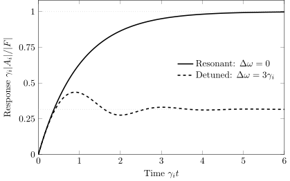
Quantitative solution of $\dot A_i+\gamma_i A_i=F e^{-i\Delta\omega t}$ for constant $F$, $\gamma_i\gt0$, and $A_i(0)=0$. Resonance approaches $\gamma_i|A_i|/|F|=1$; detuning $\Delta\omega=3\gamma_i$ approaches $1/\sqrt{10}$. These are reduced-equation curves, not a merger simulation or a prediction including parent depletion.

Gauge-invariant evidence

Nonlinear mixing can also be manufactured by a nonlinear coordinate transformation. A reliable claim uses asymptotic radiation multipoles, curvature scalars in a fixed tetrad prescription, or quasi-local horizon multipoles. It verifies amplitude scaling:

$$|A_i^{(2)}|\propto|A_jA_k|$$

as the parent amplitude is reduced. A spectral line whose amplitude scales linearly is likely leakage of a linear mode; one scaling quadratically supports second-order generation.

To resolve a nonzero frequency mismatch, the spectral bin width must be smaller than that mismatch. Windowing, finite signal duration, and a drifting background can broaden peaks. For a damped transient, fitting one extra sinusoid is not proof of a nonlinear normal mode. Check the angular selection rule, phase relation, amplitude scaling, and energy transfer together.

Limits of the mode picture

Modes assume a background and a projection. During a violent encounter, the geometry may change on the oscillation time, so instantaneous frequencies and eigenfunctions are ambiguous. The expansion becomes controlled again only when a small parameter and an overlap interval can be demonstrated. Strong finite-amplitude dynamics can still show energy transfer, but describing it as a resonance requires that controlled separation.

Material modes introduce additional closure and dissipation. This page treats their frequencies and couplings as inputs; it does not compute an equation of state.

Check the selection rules

Two even-parity scalar harmonics have $(\ell_1,m_1)=(2,2)$ and $(\ell_2,m_2)=(2,-1)$. Which $m$ and $\ell$ values can appear in their quadratic product?

Solution

Azimuthal addition gives $m=2+(-1)=1$. The triangle rule allows $\ell=0,1,2,3,4$, but $\ell\ge|m|$ removes $\ell=0$. Even parent parities require $\ell_1+\ell_2+\ell$ even, so $\ell$ is even. The allowed daughters are therefore $(\ell,m)=(2,1)$ and $(4,1)$. Resonant growth still requires a small frequency mismatch and nonzero projected coefficient.

References

• Gleiser, Reinaldo J., Carlos O. Nicasio, Richard H. Price, and Jorge Pullin, “Second Order Perturbations of a Schwarzschild Black Hole”, Classical and Quantum Gravity 13, L117–L124, 1996. Open PDF.
• Ioka, Kunihito, and Hiroyuki Nakano, “Second and Higher-Order Quasinormal Modes in Binary Black Hole Mergers”, Physical Review D 76, 061503, 2007. Open PDF.
• Landau, Lev D., and Evgeny M. Lifshitz, Mechanics, Third Edition, §§27–30, Butterworth-Heinemann, 1976.