Kerr Horizon and Ergoregion Anatomy

Kerr requires three structures to be kept separate: the surface where the asymptotic time-translation Killing field becomes null, the null event horizon, and the curvature singularity. In Schwarzschild, only the first two coincide, at $r=2GM$; the curvature singularity is at $r=0$. For nonzero-spin Kerr they are, respectively, the angle-dependent static limit, the outer horizon, and the ring singularity. The region between the first two is the ergoregion, where remaining at fixed spatial coordinates is impossible even though outward escape can still be possible.

Helpful background. Exact Solutions of Einstein’s Equations supplies Kerr as a maximally extended solution; Causality and Global Structure supplies event and Cauchy horizons; The Einstein Equation fixes the vacuum theory; Killing Fields and Isometry Groups supplies stationarity and axial symmetry; and Black-Hole Geometry and Mechanics orients the horizon definitions.

Two Killing fields and the horizon roots

Consider the four-dimensional, asymptotically flat Kerr vacuum solution with physical mass $M\gt0$ and angular momentum $J$. Define

$$a\equiv\frac{J}{M}, \qquad \Sigma=r^2+a^2\cos^2\theta, \qquad \Delta=r^2-2GMr+a^2.$$

The parameter $a$ has dimensions of length. Kerr has two commuting Killing fields: $\xi=\partial_t$, normalized as a unit time translation at infinity, and $\psi=\partial_\phi$, normalized so that its orbits have period $2\pi$. Zeros of $\Delta$ occur at

$$r_\pm=GM\pm\sqrt{G^2M^2-a^2}.$$

For $0\lt\lvert a\rvert\lt GM$, the outer root $r_+$ is the future event horizon of the selected asymptotic end and the inner root $r_-$ is a Cauchy horizon in the idealized maximal extension. At the Schwarzschild endpoint $a=0$, $r_+=2GM$ is the horizon while the formal lower root $r_-=0$ is the central curvature singularity, not a horizon. At $\lvert a\rvert=GM$ the two positive roots merge into a degenerate horizon. For $\lvert a\rvert\gt GM$, the exact Kerr family has no horizon shielding its singularity; this parameter classification is not a theorem that regular collapse can overspin a black hole.

Boyer–Lindquist metric components are singular at regular horizon roots of $\Delta=0$, but curvature invariants remain finite there. Horizon-penetrating Kerr coordinates remove that chart singularity. On the rotating branch $a\ne0$, by contrast, $\Sigma=0$ means $r=0$, $\theta=\pi/2$, and curvature diverges at the ring singularity. At $a=0$, $\Sigma=r^2$ and the singularity is the Schwarzschild central locus $r=0$. Visser 2009, §9, especially eqs. (103)–(104) develops this root and regularity distinction.

Horizon generator and angular velocity

The asymptotic time translation $\xi$ is not itself normal to the rotating horizon. The null generator is the Killing combination

$$\chi=\xi+\Omega_H\psi,$$

with

$$\Omega_H=\frac{a}{r_+^2+a^2} =\frac{a}{2GMr_+}.$$

The second equality follows from $\Delta(r_+)=0$. It is a useful algebraic check because it would fail if a factor of $G$ or the definition of $a$ were changed inconsistently. The vector $\chi$ is null on $r=r_+$ and tangent to its null generators. Thus a generator advances in azimuth as it advances in asymptotic time; the horizon rotates rigidly with angular velocity $\Omega_H$ in this normalization.

For the same generator, the outer surface gravity and area are

$$\kappa_+=\frac{r_+-r_-}{2(r_+^2+a^2)}, \qquad \mathcal A_+=4\pi(r_+^2+a^2)=8\pi GMr_+.$$

Both reduce to their Schwarzschild values as $a\to0$. Surface gravity tends to zero as the two roots merge, while the area remains finite. The stationary generator and its role in the mass formula are treated in Bardeen, Carter, and Hawking 1973, pp. 162–166.

Static limit and ergoregion

The outer static limit is defined by the vanishing norm of the specifically normalized time-translation Killing field:

$$\xi^2=g_{tt}=0, \qquad r_{\mathrm E}(\theta) =GM+\sqrt{G^2M^2-a^2\cos^2\theta}.$$

This is not a null horizon generated by $\xi$. For nonzero spin, away from the rotation axis, $r_{\mathrm E}(\theta)\gt r_+$. In the region

$$r_+\lt r\lt r_{\mathrm E}(\theta),$$

the vector $\xi$ is spacelike. A worldline tangent to $\partial_t$ would be spacelike, so no physical observer can remain at fixed $(r,\theta,\phi)$. Timelike observers must rotate in the same broad sense as the hole, though a range of angular velocities is allowed outside the horizon. This is the ergoregion. At $a=0$, however, $r_{\mathrm E}(\theta)=r_+=2GM$ for every angle, so no ergoregion remains.

For nonzero spin, the static limit meets the horizon at the poles, where $\cos^2\theta=1$, and lies at $r_{\mathrm E}=2GM$ at the equator. Those two checks show immediately that the rotating static limit is not a constant-$r$ surface. Visser gives the invariant Killing-field characterization and the angle-dependent surface in Visser 2009, §§10–11.

The two panels below place the algebraic root regimes beside an exact representative meridional section. In the lower panel, inspect where the stationary limit touches the horizon and where the gray ergoregion remains between them; do not read the coordinate curves as proper distances.

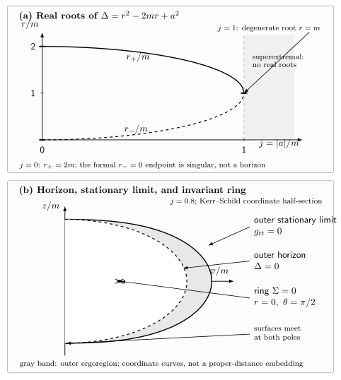
For positive-mass Kerr, $r_\pm=m\pm\sqrt{m^2-a^2}$ are real only for $j=\lvert a\rvert/m\leq1$; the $j=0$ endpoint $r_-=0$ is the Schwarzschild singularity, not a horizon. The lower panel gives exact Kerr–Schild coordinate curves at $j=0.8$: the outer stationary-limit surface bounds the gray ergoregion outside the outer horizon and meets that horizon only at the poles, while $\Sigma=0$ is the ring at $\varpi=\lvert a\rvert$, $z=0$. These are coordinate curves, not a proper-distance embedding.

A stationary circular worldline at fixed $r$ and $\theta$ has tangent proportional to

$$u\propto\xi+\Omega\psi.$$

It can represent an observer only when its norm is negative:

$$g_{tt}+2\Omega g_{t\phi}+\Omega^2g_{\phi\phi}\lt0.$$

At any exterior point where such observers exist, this quadratic inequality allows an interval of angular velocities. Far away, zero lies in that interval and a static observer is possible. Crossing the outer static limit removes $\Omega=0$ from the allowed interval, but other angular velocities remain timelike. Approaching the event horizon causes the two endpoints of the interval to converge to $\Omega_H$. This provides an operational way to see both distinctions: the static limit forbids one particular stationary motion, whereas the horizon forces every stationary limiting motion to corotate with its generator.

Frame dragging therefore should not be pictured as a material medium carrying objects around. It is a statement about the orientation of local causal cones relative to Killing coordinates. Freely falling observers cross the static limit and, in regular coordinates, the horizon without a singular force. What changes at the static limit is which Killing combinations can be timelike; what changes at the horizon is the global possibility of sending signals back to the selected future null infinity.

The ergoregion is not the black-hole interior. Events in it can still send signals to future null infinity, and suitable trajectories can exit it. Its importance is energetic: because $\xi$ is spacelike, the conserved Killing energy $E=-p\cdot\xi$ need not be positive there. Penrose extraction and wave superradiance exploit that fact, but their dynamics are developed later.

Inner horizon and scope of the exact extension

On the rotating subextremal branch $0\lt\lvert a\rvert\lt GM$, the inner root $r_-$ is also a Killing horizon in the stationary metric. In the maximal analytic extension it bounds a region beyond which the exterior initial data cease to determine a unique continuation, so it is a Cauchy horizon. This is a global role, not a statement obtained merely from solving $\Delta=0$. At $a=0$, the lower algebraic root instead lies at the central curvature singularity.

The exact rotating extension also contains additional asymptotic regions and, beyond the ring, sectors with causal pathologies. Those features help classify the solution but should not be mistaken for a prediction that a rotating star’s interior settles to the unperturbed Kerr continuation. The strong blueshift near the inner horizon makes stability a separate dynamical question.

The outer anatomy is more robustly mechanics-ready: the selected asymptotic end fixes $\xi$, axial periodicity fixes $\psi$, and regularity fixes the combination $\chi$. This is why $r_+$, $\Omega_H$, $\kappa_+$, and $\mathcal A_+$ recur in stationary laws even when the deep interior is left out of scope.

Check horizon against static limit

Take $a=(\sqrt3/2)GM$. Find $r_\pm$, the outer static-limit radii at the pole and equator, $\Omega_H$, and $\kappa_+$. Use the result to explain why the ergosurface cannot be identified with the event horizon.

Solution

Here $\sqrt{G^2M^2-a^2}=GM/2$, so $r_+=3GM/2$ and $r_-=GM/2$. At either pole, $r_{\mathrm E}=r_+=3GM/2$, whereas at the equator $r_{\mathrm E}=2GM$. Since $r_+^2+a^2=3G^2M^2$,

$$\Omega_H=\frac{\sqrt3}{6GM}, \qquad \kappa_+=\frac{1}{6GM}.$$

The event horizon has constant Boyer–Lindquist radial-coordinate location $r_+$ in this chart and is generated by $\chi=\xi+\Omega_H\psi$. The static limit is angle-dependent and defined by $\xi^2=0$. Their intersection at the poles is a special geometric coincidence, not equality of the two surfaces.

Kerr–Newman Horizon Data next combines charge and rotation into one mechanics-ready set of horizon quantities.

References

• Bardeen, James M., Brandon Carter, and Stephen W. Hawking. “The Four Laws of Black Hole Mechanics.” Communications in Mathematical Physics 31 (1973): 161–170. DOI.
• Visser, Matt. “The Kerr Spacetime: A Brief Introduction.” In The Kerr Spacetime, edited by David L. Wiltshire, Matt Visser, and Susan M. Scott. Cambridge: Cambridge University Press, 2009. arXiv:0706.0622v3.