Komar Identities and Bulk Contributions

A Komar integral becomes useful when it is moved from one boundary to another. The Killing identity and Stokes’ theorem turn that displacement into a volume integral of Ricci curvature; the Einstein equation then identifies matter, electromagnetic, and cosmological contributions. In $\Lambda=0$ vacuum the bulk term vanishes, but with sources or a cosmological term it is part of the charge relation rather than an optional correction. Tracking the trace reversal and boundary orientation is the central calculation.

Required background. Variational and Symplectic Geometry supplies conserved surface forms. Helpful background. Exact Spacetimes supplies source-free and electrovacuum checks; Causality and Global Structure supplies the hypersurface and its ends; Einstein Equations converts curvature to sources; Gravitational Actions and Boundary Terms fixes boundary orientations; Black-Hole Geometry and Mechanics supplies the horizon generator.

The differential identity behind Komar charges

Let $\xi^a$ be a Killing field and $\xi=\xi_a dx^a$ its metric-dual one-form. The Killing equation and curvature commutator give

$$\nabla_a\nabla^a\xi^b=-R^b{}_c\xi^c.$$

Equivalently, the exterior derivative of the two-form $\star d\xi$ is fixed by the Ricci contraction with $\xi$. In the site’s orientation convention, define the Komar surface functional

$$K_S[\xi]\equiv-\frac{1}{8\pi G}\int_S\star d\xi.$$

For a time translation normalized to unit norm at an asymptotically flat end, $K_{S_\infty}[t]=M$. For an axial Killing field with $2\pi$-periodic orbits,

$$J=\frac{1}{16\pi G}\int_{S_\infty}\star d\phi.$$

The different factors in these two definitions are the origin of the coefficient $-2\Omega_HJ$ below; it is not an arbitrary feature of the Smarr formula.

Now integrate over an oriented spacelike hypersurface $\Sigma$ bounded by a sphere $S_\infty$ and an inner cross-section $B$. Its oriented boundary is $\partial\Sigma=S_\infty\cup(-B)$: the outward normal at the inner boundary points into the excised interior, opposite to the direction toward infinity. The Killing identity, Stokes’ theorem, and the Einstein equation give

$$K_{S_\infty}[\xi]-K_B[\xi] =2\int_\Sigma \left(T_{ab}-\frac12Tg_{ab} +\frac{\Lambda}{8\pi G}g_{ab}\right) n^a\xi^b\,dV.$$

Here $n^a$ is the future unit normal to $\Sigma$, and ordinary matter excludes the cosmological term already shown separately. The sign is checked by a stationary perfect-fluid star: for $\Lambda=0$ and $\xi^a$ parallel to the static observers, the integrand becomes the redshifted active density $\rho+3p$. A convention change for the binormal or for which surface is subtracted must change both sides together.

Wald 1984, § 11.2, Eqs. (11.2.6)–(11.2.10), pp. 288–289 derives the surface-to-volume identity in the $G=1$ convention. The diagram below packages the sign and normalization bookkeeping. Inspect the two outward-normal arrows first: their opposite directions produce the inner minus sign. Then read the lower boxes from the horizon boundary, through the bulk, to infinity.

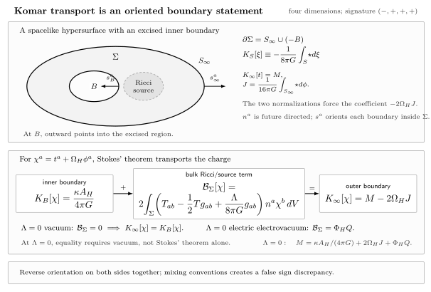
The annulus is a schematic projection of a spacelike hypersurface $\Sigma$ with $\partial\Sigma=S_\infty\cup(-B)$. With $K_S[\xi]=-(8\pi G)^{-1}\int_S\star d\xi$ and $\chi^a=t^a+\Omega_H\phi^a$, the inner orientation gives $K_\infty[\chi]-K_B[\chi]=\mathcal B_\Sigma[\chi]$, where the displayed bulk term is the trace-reversed matter contribution plus the cosmological term. For $\Lambda=0$, vacuum gives equality of the two surface charges, whereas a purely electric, source-free Maxwell exterior reorganizes the bulk as $\Phi_HQ$. The drawing is not to scale and does not represent a spacetime or conformal diagram.

The trace-reversed combination is forced by the field equation,

$$R_{ab}=8\pi G\left(T_{ab}-\frac12Tg_{ab}\right)+\Lambda g_{ab}.$$

Using $T_{ab}$ alone would miss pressure and would fail the perfect-fluid check. Treating $\Lambda$ as a stress tensor gives the same displayed term; listing it separately makes clear why asymptotically flat Komar formulas cannot simply be reused in de Sitter or AdS.

Stationary rotation and two boundary charges

For a rotating black hole, apply the identity to

$$\chi^a=t^a+\Omega_H\phi^a,$$

where $t^a$ is unit normalized at the asymptotic end and $\phi^a$ has $2\pi$-periodic orbits. The infinity integral is

$$K_\infty[\chi]=M-2\Omega_HJ.$$

On a nondegenerate bifurcation surface, the corresponding inner integral is

$$K_B[\chi]=\frac{\kappa A_H}{4\pi G}.$$

Thus matter or cosmological curvature between the horizon and infinity gives

$$M-2\Omega_HJ-\frac{\kappa A_H}{4\pi G} =2\int_\Sigma \left(T_{ab}-\frac12Tg_{ab} +\frac{\Lambda}{8\pi G}g_{ab}\right) n^a\chi^b\,dV.$$

In a stationary asymptotically flat vacuum region, the right-hand side vanishes and the vacuum Smarr formula follows. Bardeen, Carter, and Hawking perform the stationary mass-formula construction in Bardeen, Carter, and Hawking 1973, pp. 163–166, Open PDF. Wald 1984, § 12.5, Eqs. (12.5.32)–(12.5.37), pp. 334–335 makes the inner-boundary contribution explicit. Restoring $G$ gives the normalizations used here. The equation is a geometric identity for the specified Killing field; it is not yet the variational first law.

Electromagnetic bulk becomes boundary work

For the rationalized Maxwell action, the stress tensor is traceless in four dimensions,

$$T^{\mathrm{EM}}_{ab} =F_{ac}F_b{}^c-\frac14g_{ab}F_{cd}F^{cd}, \qquad T^{\mathrm{EM}}=0.$$

Assume $\Lambda=0$, stationarity up to a gauge transformation, no charged matter in the exterior, and a purely electric sector admitting the displayed potential. Maxwell’s equations and integration by parts convert its bulk term into an electric potential difference times the conserved flux charge. The resulting four-dimensional Einstein–Maxwell mass relation is

$$M=\frac{\kappa A_H}{4\pi G} +2\Omega_HJ+\Phi_HQ.$$

The potential is referenced between horizon and infinity, $\Phi_H=-\chi\cdot A|_H+\chi\cdot A|_\infty$. This conversion requires the Maxwell equations, stationarity, regularity of the horizon potential, and the declared charge normalization. A current or additional boundary leaves an extra source or boundary term.

Magnetic charge is not obtained by pretending that one globally smooth electric potential covers the magnetic bundle. A patchwise or dual-potential treatment supplies its own horizon-potential term; the one-potential formula above deliberately tests the purely electric sector.

Reissner–Nordström provides a sharp check. With $r_++r_-=2GM$ and $r_+r_-=GQ^2/(4\pi)$,

$$A_H=4\pi r_+^2, \qquad \kappa=\frac{r_+-r_-}{2r_+^2}, \qquad \Phi_H=\frac{Q}{4\pi r_+}.$$

Then

$$\frac{\kappa A_H}{4\pi G}+\Phi_HQ =\frac{r_+-r_-}{2G}+\frac{r_-}{G} =\frac{r_++r_-}{2G}=M.$$

This calculation distinguishes the electromagnetic contribution from a $\Lambda=0$ vacuum equality of Komar surfaces.

Cosmological and other bulk terms

When $\Lambda\ne0$, the volume integral generally depends on the hypersurface and the reference subtraction used to define finite charges at infinity. In extended black-hole mechanics it can be reorganized as a pressure–volume term, with $P=-\Lambda/(8\pi G)$, but that interpretation presupposes a phase space in which $\Lambda$ varies. At fixed $\Lambda$, it remains a coupling in the field equation and affects both the solution and charge definition.

Scalar potentials, non-Abelian fields, conical defects, and inner boundaries similarly alter the source or boundary content. Stokes’ theorem never says that two surface integrals are equal in isolation; it says their oriented difference equals the integral of the exterior derivative between them. Iyer and Wald formulate the more general Noether-current version, including constraints and boundary terms, in Iyer and Wald 1994, §§2–4, pp. 848–857.

Recover the charged mass relation

Use the Reissner–Nordström data above to verify the mass formula and take the uncharged limit. What does this test reveal about a missing factor of $4\pi$ in the electric potential?

Solution

Substitution gives $\kappa A_H/(4\pi G)=(r_+-r_-)/(2G)$ and $\Phi_HQ=Q^2/(4\pi r_+)=r_-/G$. Their sum is $(r_++r_-)/(2G)=M$. When $Q\to0$, $r_-\to0$ and $r_+\to2GM$, so the electric term disappears and the Schwarzschild relation remains. If one wrote $\Phi_H=Q/r_+$ while retaining the rationalized charge used in the horizon equation, the electric term would be too large by $4\pi$ and the identity would fail. Charge and potential conventions must be paired.

Smarr Relations from Scaling derives the same algebraic relation from homogeneity and shows when new scales change it.

References

• Bardeen, James M., Brandon Carter, and Stephen W. Hawking. “The Four Laws of Black Hole Mechanics.” Communications in Mathematical Physics 31 (1973): 161–170. DOI.
• Iyer, Vivek, and Robert M. Wald. “Some Properties of Noether Charge and a Proposal for Dynamical Black Hole Entropy.” Physical Review D 50 (1994): 846–864. DOI.
• Wald, Robert M. General Relativity. Chicago: University of Chicago Press, 1984. DOI.