Physical-Process First Law

The physical-process first law asks what a stationary horizon does when a small amount of matter actually falls through it. If the disturbance is weak enough that the event horizon remains close to a Killing horizon and the black hole settles to another stationary state, the stress-energy flux fixes the first-order area change. This is a classical, linear-response statement. It does not identify area with entropy, and it does not describe a violent merger or an arbitrary finite transition.

Required background. The Einstein Equation supplies the field equation that converts null curvature into stress-energy.

Helpful background. Exact Solutions of Einstein’s Equations supplies stationary backgrounds; Causality and Global Structure supplies the event-horizon generators and their endpoints; Flat-Background Hilbert Stress-Energy from Metric Variation supplies the flux tensor; and Black-Hole Geometry and Mechanics supplies surface gravity and horizon area.

Linearized focusing on a Killing horizon

Let the unperturbed spacetime contain a nondegenerate bifurcate Killing horizon generated by

$$\chi^a=t^a+\Omega_H\phi^a,$$

with surface gravity $\kappa\gt0$. Choose a future-directed affinely parametrized generator $k^a$ and an affine parameter $\lambda$ that vanishes at the bifurcation surface. Along the future horizon,

$$\chi^a=\kappa\lambda k^a.$$

The background expansion and shear vanish. Now perturb the black hole by a small stress-energy flux of order $\epsilon$. Assume the perturbation is regular, the horizon acquires no caustics or new generators in the region of interest, and the future geometry settles to a stationary horizon. To first order, the null Raychaudhuri equation and the Einstein equation give

$$\frac{d(\delta\theta)}{d\lambda} =-\delta R_{ab}k^ak^b =-8\pi G\,\delta T_{ab}k^ak^b.$$

The terms $\theta^2$ and $\sigma_{ab}\sigma^{ab}$ are quadratic because both optical scalars vanish in the background. Thus gravitational-wave absorption, which is represented by shear squared in this equation, does not appear as an independent first-order source in this matter-flux derivation.

Final stationarity supplies the teleological boundary condition $\delta\theta\to0$ after the flux has passed. Integrating backward gives

$$\delta\theta(\lambda) =8\pi G\int_\lambda^\infty \delta T_{ab}k^ak^b\,d\lambda'.$$

The expansion can therefore be nonzero before the matter reaches a chosen horizon point. That anticipation is not acausality in the local field equations; it reflects the global definition of the event horizon. Gao and Wald formulate the charged, rotating physical-process theorem and its flux identities in Gao and Wald 2001, §§2–3.

The time profile is clearest in the Killing parameter $v$. Choose its origin freely and write

$$\lambda=\lambda_0e^{\kappa v}, \qquad \widehat\theta=\kappa\lambda\,\delta\theta.$$

Because $d/dv=\kappa\lambda,d/d\lambda$ and $\chi^a=\kappa\lambda k^a$, the same linearized focusing equation becomes

$$-\frac{d\widehat\theta}{dv}+\kappa\widehat\theta =8\pi G\,\delta T_{ab}\chi^a\chi^b \equiv S(v), \qquad \widehat\theta(v)=\int_v^\infty e^{\kappa(v-v')}S(v')\,dv'.$$

The upper integration limit is the stationary future. It makes this an advanced response for the globally selected event horizon, not a retarded signal that a local detector could use to learn about future matter. Amsel, Marolf, and Virmani derive this Killing-parameter form and its area integral in Amsel, Marolf, and Virmani 2008, §II, pp. 4–6, Eqs. (2.1)–(2.9).

An exactly solvable pulse makes the distinction concrete. Put $x=\kappa v$, take $S(v)=S_0s(x)$, and define $y=\kappa\widehat\theta/S_0$. For

$$s(x)= \begin{cases} 6x(1-x),&0\leq x\leq1,\\ 0,&\text{otherwise}, \end{cases} \qquad \int_{-\infty}^{\infty}s(x)\,dx=1,$$

the final condition $y(+\infty)=0$ selects

$$y(x)= \begin{cases} (18/e-6)e^x,&x\lt0,\\ 18e^{x-1}-6(x^2+x+1),&0\leq x\leq1,\\ 0,&x\gt1. \end{cases}$$

Thus the source vanishes for $x\lt0$ while the selected horizon already has $y\gt0$. For a fixed infinitesimal generator bundle of background area $A_0$, first-order kinematics gives $d(\delta A/A_0)/dv=\widehat\theta$. The dimensionless accumulated response is therefore

$$a(x)\equiv\frac{\kappa^2}{S_0}\frac{\delta A(x)}{A_0} =\int_{-\infty}^{x}y(u)\,du, \qquad a(-\infty)=0, \qquad a(+\infty)=1.$$

The cross-section-wide result follows by integrating the expansion and source over the fixed background area element before applying the same normalization. The last equality follows either by direct integration or by integrating $-y'+y=s$: both $y(-\infty)$ and $y(+\infty)$ vanish, so the total response equals the unit pulse weight.

The three aligned curves below show what the future boundary condition does. Inspect the interval before the first dashed line: the source is exactly zero, but the selected expansion and accumulated linearized area are already positive.

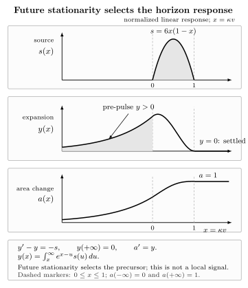
For $x=\kappa v$, the exact continuous unit pulse $s=6x(1-x)$ is supported on $0\leq x\leq1$. Final stationarity selects $y(x)=\int_x^\infty e^{x-u}s(u)\,du$, so the linearized horizon expansion is already positive before the source begins and vanishes after it ends; integrating $y$ gives a normalized accumulated area response that rises from zero to one. This pre-pulse response is future-boundary selection for a global event horizon, not a locally propagating signal from the future. The model is linear and nonextremal, assumes future settling with no caustics or new generators, and the compact pulse has derivative corners.

From stress-energy flux to area change

At first order, $d(\delta A)/d\lambda=\int\delta\theta\,dA$ on the background cross-sections. Suppose the flux has compact support away from the bifurcation surface, or falls off sufficiently fast for the integrations to converge. Interchanging the order of integration yields

$$\delta A =8\pi G\int_{\mathcal H^+} \lambda\,\delta T_{ab}k^ak^b\,d\lambda\,dA.$$

The energy associated with the horizon Killing field is

$$\delta E_\chi =\int_{\mathcal H^+} \delta T_{ab}\chi^ak^b\,d\lambda\,dA =\kappa\int_{\mathcal H^+} \lambda\,\delta T_{ab}k^ak^b\,d\lambda\,dA.$$

Consequently,

$$\boxed{\frac{\kappa}{8\pi G}\,\delta A=\delta E_\chi.}$$

For an asymptotically flat rotating black hole, conservation of the current associated with $\chi^a$ identifies the absorbed Killing energy as $\delta E_\chi=\delta M-\Omega_H\delta J$. In Einstein–Maxwell theory, with the electromagnetic gauge fixed so that the horizon-to-infinity potential difference is $\Phi_H$, the charge-current contribution gives

$$\delta M =\frac{\kappa}{8\pi G}\,\delta A +\Omega_H\delta J+\Phi_H\delta Q.$$

This has the same form as the Equilibrium First Law, but its logic is different. The equilibrium identity comes from the Hamiltonian variation of a stationary background. The physical-process proof integrates focusing and conserved flux during a perturbation. Agreement is a consistency condition, not evidence that every dynamical process is quasi-stationary.

Hypotheses that control the approximation

Small total energy alone is not sufficient. The local energy density and size of the infalling body must also be mild enough that the expansion and shear stay perturbative and no generator joins the event horizon through a caustic. Amsel, Marolf, and Virmani derive the first law and estimate the no-caustic regime for bifurcate Killing horizons in Amsel, Marolf, and Virmani 2008, §§2–3. Their analysis also shows why the qualification “quasi-stationary” carries geometric content rather than merely meaning “small energy.”

The background must be nonextremal for the affine relation $\chi^a=\kappa\lambda k^a$ with a regular bifurcation surface to provide this proof directly. The final-settling condition is essential when integrating Raychaudhuri backward. If matter violates the null energy condition, the identity can still hold at linear order, but it no longer implies a positive area change. At second order, shear, expansion squared, self-force, and backreaction enter. A merger, a topology-changing episode, or a process that adds generators is outside the theorem.

There is also a scope distinction in the charged case. The flux formula must include the electric current and the background electromagnetic field; simply inserting the total Maxwell stress tensor into the neutral derivation can double-count the work term. The gauge-invariant result uses the potential difference $\Phi_H$ and the conserved charge $Q$.

Schwarzschild transfer check

Drop a weak, neutral body of Killing energy $E$ into a Schwarzschild black hole of mass $M$, with $E\ll M$ and negligible radiation at the order being kept. Since $\kappa=1/(4GM)$, the physical-process law predicts

$$\delta A=\frac{8\pi G}{\kappa}E =32\pi G^2M E.$$

The exact stationary area is $A(M)=16\pi G^2M^2$. Expanding $A(M+E)-A(M)$ gives $32\pi G^2ME+O(E^2)$, exactly the same first-order result. The omitted $16\pi G^2E^2$ term is a useful reminder that this page proves a linear law, not the finite-difference formula.

Check your understanding

A narrow positive-energy pulse crosses an initially stationary Schwarzschild horizon. A calculation sets $\delta\theta=0$ immediately before the pulse and also imposes $\delta\theta=0$ after it. Explain why these two conditions are incompatible with the event-horizon calculation, and state the correct boundary condition.

Solution

Across the pulse, linearized Raychaudhuri gives a negative jump in $\delta\theta$ toward the future. Imposing zero expansion on both sides would therefore force the integrated positive $\delta T_{kk}$ to vanish. For an event horizon that settles down, the correct condition is $\delta\theta\to0$ in the stationary future. Integrating backward then gives a positive expansion before and during the pulse, and its integral produces $\delta A=(8\pi G/\kappa)E$. The horizon’s global location has shifted before the pulse crosses it.

Next, Third Law and Unattainability of Extremality separates the precise dynamical theorem from Nernst-like and purely geometric claims.

References

• Amsel, Aaron J., Donald Marolf, and Amitabh Virmani. “The Physical Process First Law for Bifurcate Killing Horizons.” Physical Review D 77 (2008): 024011. DOI. Open manuscript.
• Gao, Sijie, and Robert M. Wald. “The ‘Physical Process’ Version of the First Law and the Generalized Second Law for Charged and Rotating Black Holes.” Physical Review D 64 (2001): 084020. DOI.