Slicing, Foliation, and Quasi-Local Ambiguity

Quasi-local horizon data are geometric once a surface or worldtube has been specified, but the spacetime can admit several such surfaces and a numerical slicing can select different ones. This is not one undifferentiated “gauge dependence.” The expansion signs and area of a fixed two-surface are invariant under coordinate changes; apparent-horizon selection depends on a Cauchy slice; a chosen spacelike dynamical horizon has a unique marginal foliation once the fixed-tube theorem’s hypotheses are met; and competing marginal tubes can coexist. As of 2026-08-31, generic control of branch changes across binary mergers remains an open question.

If the horizon classes themselves are unfamiliar, first use Dynamical Horizons and Cross-Definition Maps. This page begins one step later by asking which surface, slice, or tube a comparison holds fixed.

Required background. Hypersurface Normals and Tangential Projectors supplies slice normals, the codimension-two screen projector, and paired null rescalings. Helpful background. Exact Spacetimes supplies controlled counterexamples; Causality and Global Structure supplies foliation-independent event horizons; Einstein Equations relates signature to flux; Black-Hole Geometry and Mechanics supplies the horizon classes; Variational and Symplectic Geometry supplies invariant charges and fluxes on a selected boundary.

Four choices that must be separated

Let $S$ be a closed spacelike two-surface. Once $S$, its outward direction, and future null normals are geometrically specified, the statements

$$\theta_{(\ell)}=0, \qquad \theta_{(n)}\lt0$$

are invariant under spacetime coordinate changes and positive null boosts. Explicitly, for $f\gt0$,

$$\ell^a\mapsto f\ell^a, \qquad n^a\mapsto f^{-1}n^a,$$

so $\theta_{(\ell)}\mapsto f\theta_{(\ell)}$ and $\theta_{(n)}\mapsto f^{-1}\theta_{(n)}$. The numerical values rescale, but zero and sign do not. Likewise, the area, intrinsic scalar curvature, Maxwell flux, and a properly normalized axial angular momentum are properties of that fixed surface.

A slicing choice selects a family of spacelike Cauchy hypersurfaces $\Sigma_t$. An apparent horizon is normally the outer boundary of a trapped region within one $\Sigma_t$, so changing the slicing can change whether it exists and which surface is outermost.

A tube choice selects a three-dimensional hypersurface $H$ formed from marginal leaves. More than one marginal tube can pass through the same region, especially near formation or merger. A horizon finder that reports only the outermost leaf can switch from one branch to another.

A foliation choice asks how one fixed tube $H$ is decomposed into marginal leaves. For one fixed smooth spacelike dynamical horizon in four dimensions, foliated by smooth closed connected marginally trapped surfaces with $\theta_{(\ell)}=0$ and $\theta_{(n)}\lt0$, that marginal foliation is unique. Thus “quasi-local horizons are foliation dependent” is too crude: multiplicity of tubes and slice selection can coexist with uniqueness of the marginal foliation on each fixed smooth spacelike tube. Ashtekar and Galloway prove this fixed-tube result in Ashtekar and Galloway 2005, §3, Corollary 3.2. It neither selects one tube from several admissible dynamical horizons nor supplies a corresponding foliation-uniqueness theorem for a null isolated horizon.

The figure separates the two operations that the word “foliation” can blur. In panel (a), read horizontal position only as outward ordering within each slice, compare the filled selected markers, and follow the dotted finder report; the branch graph is not a spacetime diagram, so its slopes say nothing about tube signature. In panel (b), instead hold one spacelike dynamical horizon fixed and inspect its marginal leaves.

Here a weakly trapped surface is a smooth, closed, connected, spacelike two-surface whose two future null expansions are everywhere nonpositive. This is broader than a marginal leaf, for which the outgoing expansion vanishes and the ingoing expansion is strictly negative.

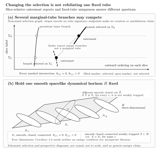
Panel (a) is a schematic branch-selection graph, not a causal or spacetime diagram. Every marked point represents a closed surface with $\theta_{(\ell)}=0$ and $\theta_{(n)}\lt0$; on each displayed slice the filled point is outermost while an unselected inner marginal surface coexists. The dotted connection records successive finder output and is not a smooth marginal tube. Shown branch endpoints are plot-window truncations, not creation or annihilation events. The branch topology and outward ordering are illustrative and nonuniversal, and no tube signature, stability, event-horizon, generic-merger, global-existence, or slicing-invariance result follows from them. Panel (b) asks a different question. A weakly trapped surface is a smooth closed connected spacelike two-surface whose two future null expansions are everywhere nonpositive. Once a smooth spacelike dynamical horizon $H$ in four dimensions is fixed and is foliated by smooth closed connected marginally trapped surfaces, Ashtekar and Galloway’s theorem says that every smooth closed connected weakly trapped surface contained in $H$ is one of those leaves, so the marginal foliation is unique. Corollary 3.2 requires neither an energy condition nor asymptotic flatness. The ribbon is a perspective projection of the three-dimensional hypersurface $H$; the ovals denote closed leaves without claiming spherical topology, a literal embedding, or quantitative scale.

Fixed-boundary invariants

Suppose two coordinate descriptions identify the same geometric $S$. They must agree on

$$A[S]=\int_S\epsilon, \qquad Q[S]=\int_S\star F,$$

and on integrals of intrinsic curvature scalars. If the same normalized axial field $\varphi^a$ is used, they also agree on horizon angular momentum. A different coordinate shape of the surface is irrelevant.

For a geometrically fixed isolated horizon, sliding between its preferred cross-sections along the null generators preserves intrinsic metric, area, charge, and the isolated-horizon moments. For a fixed dynamical horizon, its area-radius balance between two leaves is invariant once the tube, leaves, orientation, field theory, geometric evolution field, and axial field are fixed. Reparametrizing their label changes the coordinate rate $dA/dt$, not the integrated change or flux.

The distinction matters for numerical comparisons. Two codes may use different time coordinates and therefore plot different $dA/dt$, yet agree on $A$ as a function of an invariant label such as accumulated flux or area radius. Conversely, matching coordinate time does not prove that they have selected the same marginal branch.

Slice dependence and branch structure

An event horizon is defined globally and does not depend on a Cauchy slicing, although its intersections with slices do. Apparent horizons are different: their outermost rule is posed within a slice. Even in a spacetime containing a black-hole event horizon, carefully chosen slices can delay or relocate the outermost marginal surface. In Wald and Iyer’s exact extended-Schwarzschild construction, smooth Cauchy surfaces approach $r=0$ while the portion of spacetime to their past contains no outer trapped surface. This does not remove the event horizon and does not prove that every marginal surface is absent on every such slicing Wald and Iyer 1991, pp. R3719–R3722.

Near binary merger, a common pair of marginal surfaces can appear together: an outer stable branch and an inner branch with different stability behavior. Additional individual and distorted inner branches may persist. Selecting the outermost surface on each slice makes the reported apparent horizon jump at common-horizon formation, while the underlying set of marginal tubes has a richer continuous branch structure. The 2025 review synthesizes current analytic and numerical evidence in Ashtekar and Krishnan 2025, §4.2 and Open Issue 7.

The stability operator is part of the data class. Its principal eigenvalue controls local persistence of a marginally outer trapped surface under deformation. In the local continuation theorem, the needed condition is strict stability: the principal eigenvalue satisfies $\lambda_0\gt0$. Nonnegative $\lambda_0$ alone is the weaker stable case and does not make the implicit-function argument invertible. See Andersson, Mars, and Simon 2005, Definitions 1–2, Lemma 2, and Theorem 1, pp. 1–3. The simpler sign $\mathcal L_n\theta_{(\ell)}$ probes one normal direction and need not capture nonspherical modes. Existence or uniqueness claims must state which stability notion, differentiability class, matter model, and boundary condition they use.

Flux statements on a selected tube

Once a dynamical horizon $H$ and two of its leaves are fixed, an area or energy balance has invariant content. Schematically,

$$\Delta E_H =\mathcal F_{\mathrm{matter}}[H] +\mathcal F_{\mathrm{grav}}[H],$$

where the gravitational term is built from horizon shear and normal-bundle data. Its value depends on the chosen geometric tube because different tubes enclose different spacetime regions. That dependence is not removed by saying the integrand is covariant.

An isolated segment has zero cross-boundary flux under its defining energy condition. A spacelike segment can carry positive classical flux; timelike segments require a different sign and matter analysis. The original “dynamical horizon” definition reserves the term for spacelike tubes. The 2025 dynamical-horizon-segment framework instead admits nowhere-null spacelike or timelike segments; the 2026 Letter using that framework derives the displayed balance laws first for the spacelike case and states that the timelike extension changes signs. See Ashtekar, Paraizo, and Shu 2026, DHS definition on p. 2, Eqs. (2)–(6) on pp. 3–4, and remark 2 on p. 4. The formulation choice must be named before comparing signature or monotonicity statements.

What a horizon diagnostic can establish

Evidence cutoff: 2026-08-31. Before applying a result, state what two calculations share: the same embedded two-surface, the same Cauchy slice, the same marginal tube, or only the same spacetime. Without this distinction, a coordinate relabeling can be confused with a change of slicing or horizon branch.

Object held fixed	Evidence status and hypotheses	What follows	Boundary of the inference
A geometrically identified embedded closed spacelike two-surface $S$, its outward direction, its future null-normal rays, and the normalization used for charges and axial fields	Geometric identity. The cited multipole construction additionally assumes a smooth, nonextremal, type-II axisymmetric isolated horizon with no matter fields on the horizon in §III.A–C.	Coordinate relabeling leaves area, intrinsic curvature, expansion zero/sign, Maxwell charge, and properly normalized angular momentum unchanged. In the isolated-horizon domain, the source multipoles are likewise diffeomorphism invariant; see Ashtekar et al. 2004, §III.A–C, Open PDF, pp. 8–16.	The conclusion begins only after $S$ has been geometrically identified. Agreement of a few scalar values does not establish that two finders selected the same surface.
One specified Cauchy slice, outer region, boundary conditions, and outermost-MOTS rule	Slice-relative definition. Wald and Iyer give an exact counterexample in four-dimensional vacuum extended Schwarzschild.	Horizon finders can be compared on that slice after their search domain and outermost rule have been matched.	The trapped-region apparent horizon, its location, and its coordinate formation time need not survive a change of slicing. The same Schwarzschild spacetime admits Cauchy surfaces approaching the singularity whose covered past contains no outer trapped surface; see Wald and Iyer 1991, pp. R3719–R3722. This does not exclude every MOTS or remove the event horizon.
A smooth four-dimensional spacetime, a smooth foliation by spacelike Cauchy surfaces $\Sigma_t$, and a smooth closed MOTS $S\subset\Sigma_0$ with principal stability eigenvalue $\lambda_0\gt0$	Local theorem for a strictly stably outermost MOTS. The continuation lasts only while strict stability persists.	A smooth marginal tube $H$ exists locally with leaves $H\cap\Sigma_t$. If the null energy condition holds, $H$ is locally achronal; if additionally $G_{ab}\ell^a\ell^b\gt0$ somewhere on $S$ or the outgoing shear is nonzero somewhere, $H$ is spacelike near $\Sigma_0$. See Andersson, Mars, and Simon 2005, Definition 2, Lemma 2, and Theorems 1–2, Open PDF, pp. 1–4.	The theorem does not cover the marginal case $\lambda_0=0$, guarantee global continuation through a loss of strict stability, or select a tube independently of the prescribed spacetime foliation.
One fixed smooth spacelike dynamical horizon $H$ in the paper’s four-dimensional setting, foliated by smooth closed connected marginally trapped surfaces with $\theta_{(\ell)}=0$ and $\theta_{(n)}\lt0$	Fixed-tube foliation-uniqueness theorem. Corollary 3.2 does not require the paper’s later “regular dynamical horizon” genericity condition, an energy condition, or asymptotic flatness.	Every smooth weakly trapped surface contained in $H$ coincides with one of its leaves; therefore the marginal foliation of this fixed $H$ is unique. See Ashtekar and Galloway 2005, §2.2 and §3, Corollary 3.2, Open PDF, pp. 6–10.	The theorem does not select $H$ from other admissible marginal tubes and is not a foliation-uniqueness theorem for a null isolated horizon.
The same horizon portion $H_{12}$, bounding leaves, orientation, field theory, and geometric evolution and axial fields	Exact nonlinear balance laws in four-dimensional general relativity. In the 2026 construction the ambient quasi-local horizon is assumed to have topology $S^2\times\mathbb R$; a dynamical segment is nowhere null, its other null expansion is nowhere zero, and its flux-genericity scalar is not identically zero on a leaf. The Letter presents the axisymmetric spacelike derivation and states the timelike extension with sign changes.	Integrated changes of the selected area, energy, and angular momentum equal the corresponding matter and gravitational fluxes; see Ashtekar and Krishnan 2002, Eqs. (14)–(20), Open PDF, pp. 3–4 and Ashtekar, Paraizo, and Shu 2026, DHS definition and Eqs. (2)–(6), Open PDF, pp. 2–4.	A coordinate rate such as $dA/dt$ is not invariant. Changing the tube, theory, orientation, admissible evolution field, or axial normalization changes the physical comparison rather than merely relabeling it.
One declared head-on, nonspinning, axisymmetric vacuum Brill–Lindquist merger family, evolved with the reported BSSN, $1+\log$, and Gamma-driver choices	Resolution-tested numerical evidence in one finite family, not a generic-merger theorem.	The calculation tracks many marginal branches, folds in time, several bifurcation or annihilation connections, and associated stability-eigenvalue crossings; see Pook-Kolb, Hennigar, and Booth 2021, Figs. 2–5, Open PDF, pp. 3–5.	Some curves terminate numerically, and the proposed annihilation of $S_1$ with $S_1^\ast$ was not fully resolved. Universality across spinning or precessing binaries, matter models, gauges, finders, or unlocated branches remains open; see Ashtekar and Krishnan 2025, §4.2 and Open Issue 7.

The matrix does not select one slicing as the uniquely “physical” slicing. Different surfaces answer different finite-boundary questions. For a numerical cross-slicing comparison, report the dimension and field theory; initial and boundary data; lapse and shift; surface definition and outermost rule; all branches sought; stability operator and spectrum; evolution-field and axial normalizations; geometric leaf-matching rule; resolution, convergence, and known finder failures.

A theorem controlling existence, signature, and branching across slicing changes, or a converged multi-code comparison that geometrically matches tubes across a broad generic initial-data class, would trigger revision of this assessment.

For implementation details, continue to Apparent-Horizon Finding and Quasi-Local Horizon Quantities. For the physical interpretation of branch changes, use Transitions, Jumps, and Multiple Horizons. In every comparison, name the object held fixed and label the conclusion as a geometric identity, theorem, numerical result, or open problem.

Diagnose two disagreeing simulations

Two simulations evolve the same initial data with different lapse and shift. Their outermost-horizon coordinate radii and formation times disagree, but their late-time areas and quasi-local angular momenta agree. What can and cannot be concluded, and what comparison would be decisive?

Solution

Coordinate radius is not invariant, and coordinate formation time depends on the slicing. Agreement of late-time area and angular momentum is evidence that the settled surfaces approach the same geometric horizon data only after the leaves have been geometrically matched, the same charge definition and axial field have been used, and resolution uncertainty is controlled. It does not show that the earlier outermost leaves belong to the same marginal tube or that their branch transitions agree. A decisive comparison would geometrically match leaves using invariant intrinsic data, report the stability spectra and all relevant marginal branches, compare integrated flux between matched leaves, and demonstrate resolution convergence. The event horizon, reconstructed from the completed future, supplies a separate slicing-independent causal comparison but does not select a unique quasi-local tube.

Ergoregions, Penrose Processes, and Energy Extraction now uses normalized stationary charges to study how rotational energy crosses a horizon.

References

• Andersson, Lars, Marc Mars, and Walter Simon. “Local Existence of Dynamical and Trapping Horizons.” Physical Review Letters 95 (2005): 111102. DOI. Open manuscript.
• Ashtekar, Abhay, and Badri Krishnan. “Dynamical Horizons: Energy, Angular Momentum, Fluxes, and Balance Laws.” Physical Review Letters 89 (2002): 261101. DOI. Open PDF.
• Ashtekar, Abhay, and Badri Krishnan. “Quasi-Local Black Hole Horizons: Recent Advances.” Living Reviews in Relativity 28 (2025): article 8. DOI.
• Ashtekar, Abhay, and Gregory J. Galloway. “Some Uniqueness Results for Dynamical Horizons.” Advances in Theoretical and Mathematical Physics 9 (2005): 1–30. DOI. Open manuscript.
• Ashtekar, Abhay, Daniel E. Paraizo, and Jonathan Shu. “Thermodynamics of Black Holes, Far from Equilibrium.” Physical Review Letters 136 (2026): 251405. DOI. Open manuscript.
• Ashtekar, Abhay, Jonathan Engle, Tomasz Pawlowski, and Chris Van Den Broeck. “Multipole Moments of Isolated Horizons.” Classical and Quantum Gravity 21 (2004): 2549–2570. DOI. Open PDF.
• Pook-Kolb, Daniel, Robie A. Hennigar, and Ivan Booth. “What Happens to Apparent Horizons in a Binary Black Hole Merger?” Physical Review Letters 127 (2021): 181101. DOI. Open manuscript.
• Wald, Robert M., and Vivek Iyer. “Trapped Surfaces in the Schwarzschild Geometry and Cosmic Censorship.” Physical Review D 44 (1991): R3719–R3722. DOI.