Angular Teukolsky Equation and Separation Constants

Rotation deforms spin-weighted spherical harmonics into spin-weighted spheroidal harmonics. The deformation is controlled by $c=a\omega$, so the angular eigenvalue must be recomputed whenever a Kerr mode frequency changes. This page derives the pole conditions, the spherical limit, and the first rotational changes in both the eigenvalue and eigenfunction. It then explains why a generic complex-frequency mode needs an adjoint or bilinear angular pairing rather than ordinary Hermitian orthogonality.

Required background. Frames, Coframes, and Anholonomy supplies spin rotations of the complex null dyad and hence the meaning of spin weight.

Helpful background. Black-Hole Geometry and Mechanics supplies Kerr parameters and axial symmetry; PDEs and Green Functions for Gravitation supplies Sturm–Liouville theory and spectral boundary conditions; Formulations of General Relativity supplies tetrad and harmonic reductions.

From separation to the angular eigenproblem

Begin with one mode of the separated Teukolsky field,

$$\psi_s=R_{s\ell m\omega}(r) S_{s\ell m}(\theta;c)e^{-i\omega t+im\phi}, \qquad c=a\omega,$$

where $a=J/M$ is the Kerr spin parameter, $\omega$ is the possibly complex frequency, and $S$ is the polar factor. The separation itself is derived on Derivation of the Teukolsky Equation. For the integer-spin bosonic sectors considered here, $s=0,\pm1,\pm2$ and $m\in\mathbb Z$. The angular equation is

$$\frac{1}{\sin\theta}\frac{d}{d\theta} \left(\sin\theta\frac{dS}{d\theta}\right) +\left[ c^2\cos^2\theta-2cs\cos\theta -\frac{(m+s\cos\theta)^2}{\sin^2\theta} +\Lambda_{s\ell m}(c) \right]S=0.$$

Regularity at both poles quantizes $\Lambda$. At $c=0$, the regular branches are labeled by $\ell\ge\max(|m|,|s|)$. We retain that $\ell$ label by continuous or analytic continuation as $c$ changes; at finite $c$ it is a branch label, not an exactly conserved total angular momentum.

For real $c$, choose unit polar norm,

$$\int_0^\pi S_{s\ell m}(\theta;c)^* S_{s\ell' m}(\theta;c) \sin\theta\,d\theta =\delta_{\ell\ell'}$$

and fix the remaining phase near $c=0$ by a positive real overlap with the spherical mode. Farther along the real axis, positive overlap between successive modes prevents arbitrary sign jumps. This is the normalization used by the chapter’s source-projection page. A full-sphere unit mode is $S(\theta;c)e^{im\phi}/\sqrt{2\pi}$.

One eigenvalue and four conventions

Several standard sources shift the same angular eigenvalue before naming it. In this page’s notation,

$$A_{s\ell m}=\Lambda_{s\ell m}-s, \qquad \lambda_{s\ell m}=A_{s\ell m}+c^2-2cm.$$

The convention whose spherical limit is simply $\ell(\ell+1)$ is

$$E_{s\ell m}=\Lambda_{s\ell m}+s^2 =A_{s\ell m}+s(s+1).$$

Indeed, expanding the singular term replaces it by $-(m^2+s^2+2ms\cos\theta)/\sin^2\theta+E$.

Symbol	Where it is used	Value at $c=0$
$\Lambda$	additive constant in the displayed equation	$\ell(\ell+1)-s^2$
$A=\Lambda-s$	angular equation written with $s+A$	$\ell(\ell+1)-s(s+1)$
$E=\Lambda+s^2$	expanded singular-term convention	$\ell(\ell+1)$
$\lambda=A+c^2-2mc$	radial Teukolsky equation	$\ell(\ell+1)-s(s+1)$

The first three rows differ only by constant shifts; $\lambda$ also contains frequency-dependent shifts. In the gravitational $s=-2$ sector, confusing $\Lambda$ with $A$ already creates an error of two. Teukolsky’s angular and radial definitions appear together in Teukolsky 1973, § IV, Eqs. (4.8)–(4.10), printed p. 641. A symbol called $A$, $E$, or $\lambda$ in another source should be translated through its complete differential equation, not by its letter.

Pole regularity quantizes the spectrum

The endpoints $\theta=0,\pi$ are regular singular points. Near the north pole, set $S\sim\theta^p$. The leading equation is

$$S''+\frac1\theta S' -\frac{(m+s)^2}{\theta^2}S\simeq0,$$

so $p=\pm|m+s|$. Smoothness selects $p=|m+s|$. At the south pole, $\pi-\theta$ replaces $\theta$ and the selected exponent is $|m-s|$. It is therefore useful to factor

$$S(\theta)= \left(\sin\frac\theta2\right)^{|m+s|} \left(\cos\frac\theta2\right)^{|m-s|} y(\cos\theta),$$

where $y$ is regular on $[-1,1]$. The discarded local branches are generally singular in the tetrad component and are not restored by merely being square-integrable in a special borderline case.

When either selected exponent is zero, the second local solution is logarithmic. It can be square-integrable but is not smooth in a regular polar frame, so regularity still selects the analytic branch.

For real $c$, these endpoint conditions make the problem self-adjoint in $L^2([0,\pi],\sin\theta\,d\theta)$. To see the consequence, multiply the $\ell$ equation by $S_{\ell'}^*$, subtract the conjugated $\ell'$ equation multiplied by $S_\ell$, and integrate. The result is

$$\begin{aligned} &(\Lambda_\ell-\Lambda_{\ell'}^*) \int_0^\pi S_{\ell'}^*S_\ell\sin\theta\,d\theta\\ &\quad= \left[\sin\theta\left( S_\ell\frac{dS_{\ell'}^*}{d\theta} -S_{\ell'}^*\frac{dS_\ell}{d\theta} \right)\right]_0^\pi . \end{aligned}$$

The regular pole powers make the boundary term vanish. Setting $\ell'=\ell$ first proves that every eigenvalue is real; applying that result to two distinct eigenvalues proves orthogonality. This proof also shows why regularity, measure, and operator domain are part of the spectral problem rather than optional conventions.

Spherical limit and first corrections

At $c=0$, the equation becomes the spin-weighted spherical-harmonic equation. With the phase convention of Spin-Weighted Spherical Harmonics, the unit-polar and unit-sphere functions are related by

$$S_{s\ell m}(\theta;0)e^{im\phi} =\sqrt{2\pi}\,{}_sY_{\ell m}(\theta,\phi).$$

This is the unit-sphere normalization and phase convention of Goldberg et al. 1967, pp. 2156–2159.

The eigenvalues are

$$\Lambda_{s\ell m}(0)=\ell(\ell+1)-s^2, \qquad A_{s\ell m}(0)=\ell(\ell+1)-s(s+1).$$

For example, the lowest corotating gravitational mode has

$$S_{-2,2,2}(\theta;0) =\sqrt{\frac{5}{32}}(1+\cos\theta)^2,$$

so its north- and south-pole powers are respectively $0$ and $4$. Its four constants at $c=0$ are

$$\Lambda=2, \qquad A=4, \qquad E=6, \qquad \lambda=4.$$

This one mode checks the pole behavior, spherical eigenfunction, normalization, and every constant shift at once.

Rotation has a nonzero linear effect for generic spin-weighted modes. For $\ell>0$, let $x=\cos\theta$ and denote the unit-polar spherical function by $S^{(0)}_{s\ell m}$. In the adopted phase convention,

$$\begin{aligned} xS^{(0)}_{s\ell m}={}& C_{\ell+1}S^{(0)}_{s,\ell+1,m} -\frac{sm}{\ell(\ell+1)}S^{(0)}_{s\ell m}\\ &+C_\ell S^{(0)}_{s,\ell-1,m}, \end{aligned}$$

where

$$C_k=\sqrt{ \frac{(k^2-m^2)(k^2-s^2)}{k^2(4k^2-1)} }.$$

Terms outside the allowed range are absent. In particular, $C_\ell=0$ at a lowest allowed branch. Multiplication by $x$ is therefore tridiagonal, not purely off-diagonal: the middle term is the source of the linear eigenvalue shift. For the scalar monopole, omit the undefined diagonal and lower terms; $xS^{(0)}_{000}=C_1S^{(0)}_{0,1,0}$.

Writing the eigenproblem as $H(c)S=\Lambda(c)S$ gives

$$H(c)=H(0)+2csx-c^2x^2.$$

Ordinary nondegenerate perturbation theory then yields

$$\Lambda_{s\ell m}(c) =\ell(\ell+1)-s^2 -\frac{2ms^2}{\ell(\ell+1)}c+O(c^2),$$

for $\ell>0$. The scalar monopole instead has no linear correction. The eigenfunction changes according to

$$\begin{aligned} S_{s\ell m}(c)={}&S^{(0)}_{s\ell m}\\ &+c\left[ \frac{sC_\ell}{\ell}S^{(0)}_{s,\ell-1,m} -\frac{sC_{\ell+1}}{\ell+1}S^{(0)}_{s,\ell+1,m} \right]+O(c^2). \end{aligned}$$

An absent lower-branch term is omitted rather than evaluated at a zero denominator. The same linear shift applies to $A$ and $E$ because their differences from $\Lambda$ are constant. The eigenvalue coefficients agree with Berti, Cardoso, and Casals 2006, § II.C, Eqs. (2.13) and (2.16a)–(2.16c), printed pp. 5–6; the eigenfunction coefficients agree with Press and Teukolsky 1973, Part II, § III(a), Eqs. (3.2) and (3.7)–(3.9), printed pp. 655–656.

For $(s,\ell,m)=(-2,2,2)$, $\langle x\rangle=2/3$ and $C_2=0$, so

$$\Lambda(c)=2-\frac83c+O(c^2), \qquad \lambda(c)=4-\frac{20}{3}c+O(c^2),$$

while the full-sphere unit mode begins as

$$\frac{S_{-2,2,2}(\theta;c)e^{2i\phi}}{\sqrt{2\pi}} ={}_{-2}Y_{22} +\frac{10}{9\sqrt{35}}c\,{}_{-2}Y_{32}+O(c^2).$$

Thus rotation changes the eigenvalue at first order and mixes the angular profile toward $\ell=3$, but it never mixes $m$: axial symmetry remains exact. At $O(c^2)$, the $x^2$ term reaches two spherical multipoles away. The resulting spectral matrix and independent continued-fraction benchmark are developed on Spin-Weighted Spheroidal Harmonics.

For this mode, the unit-polar first-order shape change is $\partial_cS|_0=(2/9)(3x-2)S(x;0)$ with $x=\cos\theta$. Inspect the upper panel for the redistribution toward the north pole and the lower panel for agreement with this first-order correction. The computational companion checks both the eigenvalues and the plotted functions against an independent regular-series solution.

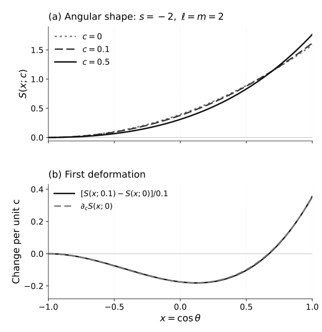
Positive real $c$ redistributes the unit-polar $(-2,2,2)$ profile toward $x=1$. The second panel compares $[S(x;0.1)-S(x;0)]/0.1$ with $\partial_cS|_0=(2/9)(3x-2)S(x;0)$. Every axis is dimensionless; $\int_{-1}^{1}S^2dx=1$ and the overlap with the spherical profile is positive. The azimuthal factor $e^{2i\phi}$ and both pole orders remain unchanged. This quantitative harmonic comparison does not specify a radiation flux.

Complex frequency, adjoints, and conjugation

For a rotating black hole, a quasinormal frequency is generically complex, so $c=a\omega$ is complex and $H(c)$ is non-Hermitian. There are important exceptions: Schwarzschild has $c=0$ even when $\omega$ is complex, and the scalar $s=0$ operator also has real coefficients for purely imaginary $c$. The statement that complex frequency destroys self-adjointness is therefore generic, not universal.

For generic complex $c$,

$$H(c)^\dagger=H(c^*)$$

on the corresponding regular domain. A right mode satisfies $H(c)S_\ell=\Lambda_\ell S_\ell$, while its Hermitian left mode is obtained from the adjoint problem. Left and right modes can be normalized biorthogonally. Because the differential expression is complex symmetric in the real $\theta$ representation, one may instead use the bilinear pairing

$$(f,g)_B=\int_0^\pi f(\theta)g(\theta)\sin\theta\,d\theta.$$

The same boundary-form subtraction, now without complex conjugation, makes right modes with distinct eigenvalues bilinearly orthogonal. For this complex-symmetric operator, the adjoint left ket may be chosen as $S^*$; with that choice, its left-right overlap is precisely $(S,S)_B$. If this self-pairing vanishes, standard biorthogonal normalization fails; at a defective eigenvalue, associated Jordan-chain functions may be needed. In particular, ordinary same-$c$ overlaps with $S^*$ must not be silently replaced by Kronecker deltas. The fixed-complex-$c$ adjoint construction and its orthogonality identity are developed in London 2023, § II, Eqs. (9)–(17), printed pp. 5–6.

The eigenvalue and eigenfunction are obtained by analytic continuation from a chosen spherical branch or by solving this non-Hermitian problem directly. An analytic phase can be continued locally from $c=0$ along a stated path. A numerical unit-norm phase convention is also possible, but it is not itself a holomorphic normalization. Near a degeneracy or branch point, track both left-right overlaps and residuals rather than sorting eigenvalues alone.

Complex conjugation gives an exact equation-level check. Under

$$(s,m,c,\Lambda) \mapsto (-s,-m,-c^*,\Lambda^*)$$

each term is unchanged: $(-c^*)^2=(c^2)^*$, $(-c^*)(-s)=c^*s$, and $(-m-s\cos\theta)^2=(m+s\cos\theta)^2$. Consistently continued branches therefore obey

$$\Lambda_{-s,\ell,-m}(-c^*) =\Lambda_{s\ell m}(c)^*.$$

With the spherical-limit phase used above, the eigenfunctions can be chosen so that

$$S_{-s,\ell,-m}(\theta;-c^*) =(-1)^{s+m}S_{s\ell m}(\theta;c)^*.$$

A different dyad or harmonic phase changes the prefactor but not the eigenvalue identity or any reconstructed physical field. Berti, Cardoso, and Casals record the complex-$c$ equation, its spherical branches, and useful symmetries in Berti, Cardoso, and Casals 2006, § II.A, Eqs. (2.1)–(2.5), printed pp. 3–4.

Closing the angular–radial loop

The radial equation contains

$$\lambda_{s\ell m}(\omega) =\Lambda_{s\ell m}(a\omega)-s+a^2\omega^2-2am\omega.$$

The dependency chain is

$$\omega\longrightarrow c=a\omega \longrightarrow\Lambda_{s\ell m}(c) \longrightarrow\lambda_{s\ell m}(\omega) \longrightarrow\text{radial boundary residual}.$$

Thus a radial quasinormal calculation is nonlinear in $\omega$ even before its boundary conditions are imposed. Holding $\lambda$ fixed while varying $\omega$ does not solve the rotating Kerr separation problem. Conversely, a high-accuracy angular eigenvalue is not a mode frequency: the ingoing/outgoing conditions on Radial Teukolsky Equation and Physical Solutions must also be satisfied. Berti, Cardoso, and Casals state this two-equation root procedure explicitly in Berti, Cardoso, and Casals 2006, § II.G, printed p. 12.

For real-frequency scattering, an end-to-end consistency loop is available: solve the angular problem with the declared norm and phase, use precisely that harmonic in the source projection, solve the radial equation, and confirm the reconstructed flux balance. Rescaling $S\mapsto qS$ requires its angular coefficient and radial amplitude to transform inversely; the final curvature and flux must be unchanged. Sasaki and Tagoshi exhibit the unit-polar normalization inside a complete $s=-2$ source and radial convention in Sasaki–Tagoshi 2003, § 2.1, Eqs. (8)–(20), printed pp. 8–9.

Common pitfalls

Using ordinary spherical harmonics at finite rotation. At $a\omega\ne0$, the angular potential contains spin-rotation terms. Spherical harmonics are then a basis for expansion, not exact separated eigenfunctions.

Dropping the diagonal $\cos\theta$ matrix element. For $s\ne0$ and $m\ne0$, multiplication by $\cos\theta$ includes $-sm/[\ell(\ell+1)]$ on the original multipole. Omitting it erases the correct $O(c)$ eigenvalue shift.

Treating $\ell$ as exact angular momentum at finite $c$. Rotation preserves $m$ but mixes spherical $\ell$ values. The spheroidal $\ell$ identifies the branch that reaches a chosen spherical mode as $c\to0$.

Assuming Hermitian orthogonality for generic quasinormal modes. Generic complex $c$ makes the angular operator non-Hermitian. Use a left-right or bilinear pairing and state its normalization.

Comparing $A$, $E$, and $\lambda$ without shifts. A disagreement by $s(s+1)$, $c^2$, or $2cm$ is often definitional. Write both complete angular and radial equations before diagnosing a physical difference.

Exercises

Verify directly that $S_{-2,2,2}(\theta;0)=\sqrt{5/32}(1+\cos\theta)^2$ has unit polar norm and that $S e^{2i\phi}/\sqrt{2\pi}$ has unit full-sphere norm. If $S\mapsto e^{i\chi}S$, how must the radial amplitude and projected source coefficient change?

Solution

With $x=\cos\theta$ and $dx=-\sin\theta\,d\theta$,

$$\int_0^\pi |S|^2\sin\theta\,d\theta =\frac5{32}\int_{-1}^{1}(1+x)^4\,dx =\frac5{32}\frac{2^5}{5}=1.$$

The azimuthal integral contributes $2\pi$, while the full-sphere mode carries $1/(2\pi)$ in its squared normalization, so its norm is also one. The separated field contains the product $RS$. Therefore $S\mapsto e^{i\chi}S$ requires $R\mapsto e^{-i\chi}R$. The coefficient of the same basis function in a projected source transforms in the same inverse way. The eigenvalue is unaffected.

Verify the conjugation map term by term. Then, for $\ell>0$, use the small-$c$ eigenvalue to show that

$$\lambda_{s\ell m}(c) =\ell(\ell+1)-s(s+1) -2m\left[1+\frac{s^2}{\ell(\ell+1)}\right]c+O(c^2).$$

Why does a radial root finder for rotating Kerr that varies $\omega$ while holding $\lambda$ fixed fail even when $|a\omega|\ll1$? Treat the scalar monopole separately.

Solution

After complex conjugation, $c^2$ becomes $(c^*)^2$ and $\Lambda$ becomes $\Lambda^*$. Replacing $(s,m,c)$ by $(-s,-m,-c^*)$ gives

$$(-c^*)^2=(c^*)^2, \qquad (-c^*)(-s)=c^*s, \qquad (-m-s\cos\theta)^2=(m+s\cos\theta)^2.$$

The transformed equation is therefore identical, which proves the stated eigenvalue symmetry for consistently labeled branches.

Since $A=\Lambda-s$ has the same linear coefficient as $\Lambda$,

$$A(c)=\ell(\ell+1)-s(s+1) -\frac{2ms^2}{\ell(\ell+1)}c+O(c^2).$$

Substitution into $\lambda=A+c^2-2mc$ gives the requested expression. A change $\delta\omega$ changes $c$ by $a\,\delta\omega$ and therefore changes $\lambda$ already at first order for generic $m$ when $a\ne0$. Holding $\lambda$ fixed then feeds the wrong potential into the radial equation. For $m=0$ the linear term vanishes, but the $O(c^2)$ dependence remains. In particular, $\Lambda_{000}=-c^2/3+O(c^4)$ and hence $\lambda_{000}=2c^2/3+O(c^4)$. The angular and radial problems are still coupled for rotating Kerr. In Schwarzschild, $a=c=0$, so this particular feedback disappears.

References

• Berti, Emanuele, Vitor Cardoso, and Marc Casals. “Eigenvalues and Eigenfunctions of Spin-Weighted Spheroidal Harmonics in Four and Higher Dimensions.” Physical Review D 73 (2006): 024013; correction 109902. DOI. Open PDF. Correction.
• Goldberg, Joshua N., A. J. Macfarlane, Ezra T. Newman, Fritz Rohrlich, and E. C. G. Sudarshan. “Spin-s Spherical Harmonics and ð.” Journal of Mathematical Physics 8 (1967): 2155–2161. DOI.
• London, Lionel T. “Biorthogonal Harmonics for the Decomposition of Gravitational Radiation. I. Angular Modes, Completeness, and the Introduction of Adjoint-Spheroidal Harmonics.” Physical Review D 107 (2023): 044056. DOI. Open PDF.
• Press, William H., and Saul A. Teukolsky. “Perturbations of a Rotating Black Hole. II. Dynamical Stability of the Kerr Metric.” Astrophysical Journal 185 (1973): 649–673. DOI.
• Sasaki, Misao, and Hideyuki Tagoshi. “Analytic Black Hole Perturbation Approach to Gravitational Radiation.” Living Reviews in Relativity 6 (2003): article 6. DOI. Open PDF.
• Teukolsky, Saul A. “Perturbations of a Rotating Black Hole. I. Fundamental Equations for Gravitational, Electromagnetic, and Neutrino-Field Perturbations.” Astrophysical Journal 185 (1973): 635–647. DOI.