Spin-Weighted Spheroidal Harmonics

For massless fields described by the Teukolsky equation, rotation deforms the angular spectrum through the dimensionless product $c=a\omega$: neither the Kerr spin parameter $a$ nor frequency $\omega$ acts alone. Spin-weighted spheroidal harmonics solve the resulting regular eigenproblem, reduce to spin-weighted spherical harmonics at $c=0$, and mix spherical multipoles at finite $c$. The practical task is to find both an eigenvalue and a normalized angular shape. Here we derive their spherical-basis representation, visualize the first deformation, and test a downloadable matrix calculation against an independent continued fraction for real and complex $c$.

Required background. Killing Fields and Isometry Groups supplies the axial quantum number; Events, Intervals, and Minkowski Geometry supplies local Lorentz and helicity conventions.

Helpful background. Black-Hole Geometry and Mechanics fixes Kerr’s parameter range; PDEs and Green Functions for Gravitation supplies spectral boundary problems; Formulations of General Relativity locates the separated angular equation within the field system; Frames, Coframes, and Anholonomy supplies the tetrad and spin-weight interpretation.

The spheroidal eigenproblem

For a separated massless bosonic Teukolsky field on Kerr, take integer spin weight $s$, integer $m$, and the angular factor $e^{im\phi}$. Here $a=J/M$ has dimensions of length, so $c=a\omega$ is dimensionless. This $c$ denotes the spheroidal parameter; it can be complex even when the Kerr geometry is real. With $x=\cos\theta$, the polar function satisfies

$$\frac{d}{dx}\left[(1-x^2)\frac{dS}{dx}\right] +\left[c^2x^2-2csx+s+A_{s\ell m}(c) -\frac{(m+sx)^2}{1-x^2}\right]S=0.$$

The $c$-dependent terms preserve axial symmetry but destroy the full rotational symmetry of the spherical problem. Thus $m$ remains an azimuthal quantum number, while $\ell$ labels the branch continued from a spherical harmonic at $c=0$. The integer $s$ describes transformation under rotation of the tangent dyad; it is not another angular-momentum index.

The domain consists of spin-weighted fields regular in smooth polar frames. In the displayed coordinate frame the regular representative has the form

$$S(x;c)=(1-x)^{|m+s|/2}(1+x)^{|m-s|/2}\,F(x;c),$$

with $F$ regular at both endpoints. The other local Frobenius solution is excluded, including the logarithmic solution when an exponent is zero. These endpoint conditions select a discrete set of eigenvalues $A$. A function satisfying the differential equation at interior grid points can still be wrong if it contains the singular endpoint solution.

The polar inner product and full angular harmonic used here are

$$\langle f,g\rangle_x=\int_{-1}^{1}f^*(x)g(x)\,dx,\qquad \langle S,S\rangle_x=1,$$ $${}_s\mathcal S_{\ell m}(\theta,\phi;c) =\frac{S_{s\ell m}(\cos\theta;c)e^{im\phi}}{\sqrt{2\pi}}.$$

Consequently the full harmonic has unit norm on the sphere. If a source instead unit-normalizes the full harmonic $\widehat S(x;c)e^{im\phi}$ over the sphere, then $S=\sqrt{2\pi}\,\widehat S$. Eigenvalues do not change under this conversion. We use the same unit-polar normalization as Berti, Cardoso, and Casals 2006, § II.B, Eq. (2.10), p. 4 and the Angular Teukolsky Equation page, which develops the endpoint and separation-constant arguments further.

At $c=0$ define the real polar basis $Y_j(x)$ by

$${}_sY_{jm}(\theta,\phi) =\frac{Y_j(\cos\theta)e^{im\phi}}{\sqrt{2\pi}}, \qquad \int_{-1}^{1}Y_jY_k\,dx=\delta_{jk}.$$

The dyad, Condon–Shortley phase, and eth signs are those of Spin-Weighted Spherical Harmonics. In particular, $ð\,{}_sY_{jm}=\sqrt{(j-s)(j+s+1)}\,{}_{s+1}Y_{jm}$. This construction and normalization descend from Goldberg et al. 1967, pp. 2155–2161.

The four common separation constants encode one eigenvalue:

Symbol	Definition here	Spherical value
$A$	Eigenvalue in the displayed equation	$\ell(\ell+1)-s(s+1)$
$\Lambda$	$A+s$	$\ell(\ell+1)-s^2$
$E$	$A+s(s+1)$	$\ell(\ell+1)$
$\lambda$	$A+c^2-2mc$	$\ell(\ell+1)-s(s+1)$

Always translate this entire dictionary before comparing numerical values. The angular operator is Hermitian for real $c$ on the regular domain; the boundary term $(1-x^2)(f^*g'-f'^*g)$ vanishes at both endpoints. For complex $c$ the same boundary conditions remain, but Hermitian orthogonality generally does not. The scalar case $s=0$ with purely imaginary $c$ is an exception: only the real coefficient $c^2$ remains, so the operator is still Hermitian. We return to the appropriate left eigenvectors below.

From spherical harmonics to a sparse matrix

Expand a single spheroidal mode as

$$S_{s\ell m}(x;c)=\sum_{j=j_0}^{\infty}b_j^{(\ell)}(c)Y_j(x), \qquad j_0=\max(|s|,|m|).$$

The coefficient $b_j^{(\ell)}=\langle Y_j,S_{s\ell m}\rangle_x$ measures the spherical $j$ component of this one spheroidal mode. Normalization gives $\sum_j|b_j^{(\ell)}|^2=1$. This is a change of angular basis: it does not imply that the underlying solution contains several independent physical modes.

Multiplication by $x$ has the real symmetric tridiagonal matrix

$$X_{jk} =C_{k+1}\delta_{j,k+1} -\frac{sm}{k(k+1)}\delta_{jk} +C_k\delta_{j,k-1},$$ $$C_k=\sqrt{\frac{(k^2-m^2)(k^2-s^2)}{k^2(4k^2-1)}}.$$

At the lower end there is no basis vector below $j_0$. Set $C_0=0$, and define the $k=0$ diagonal entry as zero in the scalar monopole case $s=m=0$. These conventions remove apparent divisions by zero. The diagonal term matters: $xY_j$ generally contains $Y_j$ as well as its neighbors.

Move the two deformation terms to the eigenvalue side of the differential equation. Orthogonal projection onto every $Y_j$ then gives

$$\mathbf H(c)\mathbf b=A\mathbf b,\qquad \mathbf H(c)=\mathbf H_0+2cs\mathbf X-c^2\mathbf X^2,$$ $$(H_0)_{jk}=[j(j+1)-s(s+1)]\delta_{jk}.$$

Multiplication by $x$ changes $j$ by at most one; multiplication by $x^2$ changes it by at most two. Hence $\mathbf H$ is pentadiagonal. For real $c$ it is real symmetric. For complex $c$ it remains symmetric under transpose, $\mathbf H^T=\mathbf H$, but is generally not Hermitian.

Project the square correctly

Let $P_J$ retain $j_0\le j\le J$, and let $\mathbf e_J$ denote the last retained unit vector. Squaring a matrix and truncating a matrix do not commute:

$$P_J\mathbf X^2P_J =(P_J\mathbf XP_J)^2+C_{J+1}^2\mathbf e_J\mathbf e_J^T.$$

The extra contribution is the path $J\to J+1\to J$ through the omitted basis vector. To obtain the Galerkin projection of the stated differential operator, construct $\mathbf X$ through $J+1$, square it, and only then crop to $j\le J$. A matrix built by squaring the already cropped $\mathbf X$ has a different final diagonal. Its error can be invisible for a very well resolved low mode, but it is not the same finite projection.

For a real symmetric matrix, the numerical solver can preserve that structure by using NumPy 2.0, numpy.linalg.eigh. For complex $c$, use a general eigensolver and explicitly check its left and right eigenvectors. The download implements both cases.

What the first admixture does

For real $c$ near zero and $\ell>0$, first-order perturbation theory gives

$$A'(0)=2sX_{\ell\ell} =-\frac{2ms^2}{\ell(\ell+1)},$$ $$b_j^{(\ell)}(c) =c\,\frac{2sX_{j\ell}}{\ell(\ell+1)-j(j+1)}+O(c^2) \quad(j\ne\ell).$$

The diagonal element shifts the eigenvalue; the off-diagonal elements change the shape. Only $j=\ell\pm1$ can appear in this first-order correction. The shift agrees with Berti, Cardoso, and Casals 2006, § II.C, Eq. (2.16b), p. 6. For a scalar, the linear deformation vanishes and the leading effect is quadratic in $c$; the scalar monopole has $A_{000}=-c^2/3+O(c^4)$.

Consider the branch used throughout the benchmark, $(s,\ell,m)=(-2,2,2)$. There is no $j=1$ spin-minus-two harmonic, so only $j=3$ contributes at first order. In the positive spherical phase,

$$Y_2(x)=\sqrt{\frac5{32}}(1+x)^2,\qquad Y_3(x)=\sqrt{\frac7{32}}(1+x)^2(3x-2),$$ $$S_{-2,2,2}(x;c) =Y_2(x)+\frac{10c}{9\sqrt{35}}Y_3(x)+O(c^2),$$ $$A_{-2,2,2}(c)=4-\frac83c-\frac{139}{189}c^2+O(c^3).$$

The shape change has the particularly simple form

$$\left.\frac{\partial S}{\partial c}\right|_{c=0} =\frac29(3x-2)Y_2(x).$$

For small positive $c$, the profile therefore grows near $x=1$ and decreases for $-1<x<2/3$. Its normalization remains one because $\langle Y_2,\partial_cS|_0\rangle_x=0$. This calculation makes precise what “deformation” means: angular amplitude is redistributed at fixed total norm. The north pole remains finite and the south pole still vanishes as $(1+x)^2$, or fourth order in angular distance from $\theta=\pi$.

Inspect the first panel for the redistribution toward the north pole. The second panel isolates the small difference and compares it with the first-order prediction; the residual separation between the curves is a higher-order correction within this angular equation.

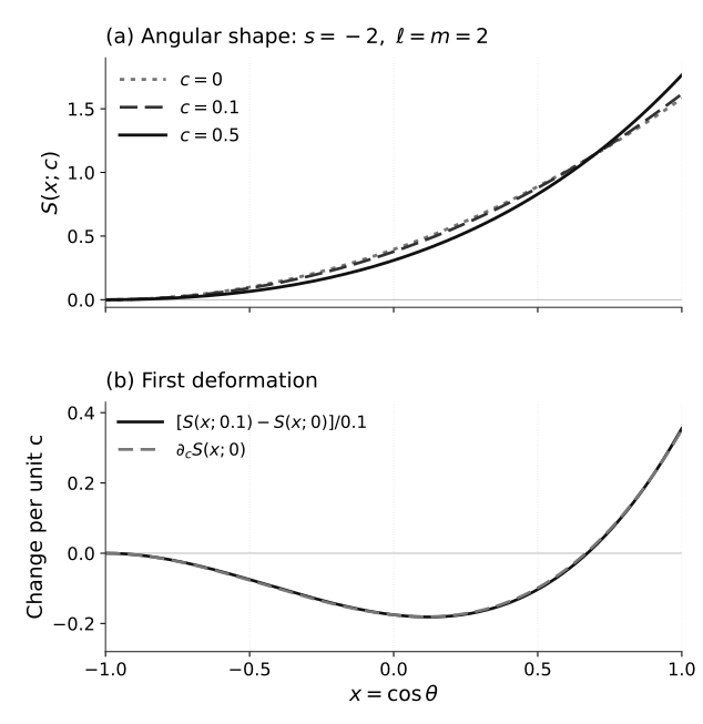
Positive real $c$ redistributes the unit-polar $(-2,2,2)$ profile toward $x=1$. The second panel compares $[S(x;0.1)-S(x;0)]/0.1$ with $\partial_cS|_0=(2/9)(3x-2)Y_2(x)$. Both axes are dimensionless; each profile has $\int_{-1}^{1}S^2dx=1$ and a common positive-overlap phase. Divide $S$ by $\sqrt{2\pi}$ for the polar factor of a unit full-sphere harmonic. This is a quantitative harmonic comparison, not a radiation-flux plot.

For a fixed real $c$, the matrix of mixing coefficients between complete spherical and spheroidal orthonormal bases is unitary. In a finite calculation, the last retained coefficients help diagnose how well a particular spheroidal mode is resolved; their norm does not directly equal the unknown infinite omitted tail. A waveform expressed in spherical multipoles can contain contributions from several spheroidal branches at the same $m$. The distinction between this basis conversion and actual coupling of field equations is developed in Mode Coupling and Broken Separability.

An independent regular-series calculation

An eigenvalue from a second representation provides a stronger check than repeating the same matrix diagonalization. For $s=-2$, $m=2$, factor both pole behaviors and expand

$$S(x;c)=N e^{cx}(1+x)^2\sum_{p=0}^{\infty}a_p(1+x)^p.$$

The constant $N$ fixes the norm and phase after the series solution is found. Substitution into the differential equation produces

$$\alpha_0a_1+\beta_0a_0=0,\qquad \alpha_pa_{p+1}+\beta_pa_p+\gamma_pa_{p-1}=0 \quad(p\ge1),$$ $$\begin{aligned} \alpha_p&=-2(p+1)(p+5),\\ \beta_p&=p(p+5)+4-(4p+6)c-c^2-A,\\ \gamma_p&=2cp. \end{aligned}$$

This is the specialization of Berti, Cardoso, and Casals 2006, § II.A, Eqs. (2.5)–(2.8), p. 3. Their erratum corrects higher small-$c$ coefficients; it is incorporated in the linked arXiv v4.

The minimal solution is the coefficient sequence that decreases relative to the other recurrence solution at large $p$. Selecting it gives

$$\beta_0-\frac{\alpha_0\gamma_1}{ \displaystyle\beta_1-\frac{\alpha_1\gamma_2}{ \displaystyle\beta_2-\cdots}}=0.$$

This condition enforces the regular solution at the second pole as well as the first. It follows from eliminating successive ratios $a_{p+1}/a_p$; see Berti, Cardoso, and Casals 2006, §§ II.A–II.B, Eq. (2.9), p. 4. The benchmark follows the lowest $\ell=2$ branch from $A(0)=4$. Higher branches require the corresponding continued-fraction inversion and independent branch identification; changing only the integer $\ell$ in this specialized program does not implement them.

At finite cutoff, evaluate the continued fraction backwards, solve its root condition, and reconstruct the minimal coefficients backwards. Direct forward recurrence may magnify a tiny admixture of the dominant solution. Increasing the cutoff and precision independently checks both truncation and roundoff. Finally normalize the series profile, match its phase to the spherical calculation, and compare functions at points that were not used to determine the matrix eigenvalue.

Track the branch and its conditioning

Start with $\mathbf b(0)=\mathbf e_\ell$. At each small step in $c$, choose the eigenvector with the largest absolute overlap with the previous one, normalize it, and remove the relative phase so that the consecutive overlap is positive real. Halve the step and increase the basis to test whether this selection is stable. The benchmark finally fixes the otherwise arbitrary overall phase by making $b_2$ positive real. At finite $c$ the label $\ell$ remembers the continuation path; sorting complex eigenvalues by their real parts cannot supply the same information.

For a simple eigenpair of the complex symmetric matrix, a left ket can be chosen as $\mathbf w=\mathbf v^*$, since $\mathbf H^\dagger\mathbf w=A^*\mathbf w$. Its pairing with the right ket is $\mathbf w^\dagger\mathbf v=\mathbf v^T\mathbf v$. With unit Euclidean norm,

$$\kappa_A=\frac{\|\mathbf w\|_2\|\mathbf v\|_2} {|\mathbf w^\dagger\mathbf v|} =\frac1{|\mathbf v^T\mathbf v|}.$$

This condition number quantifies first-order eigenvalue sensitivity to unstructured additive matrix perturbations in the Euclidean operator norm. A small right residual alone does not bound the eigenvalue error tightly when $\kappa_A$ is large. Compute the adjoint residual as well; it tests the chosen left eigenvector and pairing. The fixed-$c$ bilinear relation is the matrix counterpart of the angular construction in London 2023, § II, Eqs. (9)–(17).

For distinct eigenvalues at the same $c$, transpose symmetry gives $\mathbf v_k^T\mathbf v_\ell=0$. It does not imply $\mathbf v_k^\dagger\mathbf v_\ell=0$. Nor does it establish orthogonality between modes evaluated at different $c=a\omega_{\ell mn}$, as occurs across a Kerr QNM spectrum. A near-zero bilinear self-pairing or ambiguous overlap requires closer analysis; small-step continuation by itself is not a general exceptional-point solver.

Reproduce the eigenvalues and profiles

The Python calculation, pinned requirements, and machine-readable results contain the complete benchmark. The environment is CPython 3.9.6, NumPy 2.0.2, and mpmath 1.3.0; the optional figure uses Matplotlib 3.9.4. Save the downloads together, install the pinned requirements in that Python environment, and run:

python3 spheroidal-harmonics.py --output spheroidal-harmonics-results.json

To recompute and check the saved report without replacing it, run the same command with --check. It compares the complete report, applies explicit numerical acceptance limits, and tests that deliberately corrupted temporary reports are rejected. A failed environment, convergence, branch, norm, or comparison check exits with an error; a printed eigenvalue alone is not a pass.

The program emits the five fixed inputs, eigenvalues in the $A$ convention, basis and continued-fraction refinement, branch overlaps, matrix and adjoint residuals, normalization errors, mixing tails, condition numbers, and independent profile checks. Decimal values enter the arbitrary-precision calculation as decimal strings, so increasing its precision does not merely refine an already rounded binary input.

The cases include the exact spherical limit, two weak real deformations, one complex deformation, and the moderately larger real value $c=2$. The latter is a numerical angular test; no claim is made that it is the frequency of a particular black-hole mode. The matrix uses $J=24$; the reference continued fraction uses 80 decimal digits and cutoff 240. Both methods continue independently from $c=0$, with maximum step $0.05$.

$c$	Matrix $A$, rounded	Continued-fraction $A$, rounded
$0$	$4$	$4$
$0.1$	$3.725920378006$	$3.725920378006$
$0.5$	$2.475702761258$	$2.475702761258$
$0.3+0.1i$	$3.140114487180-0.312286681958i$	$3.140114487180-0.312286681958i$
$2$	$-4.660240022116$	$-4.660240022116$

Across these five cases, the maximum absolute matrix–fraction difference is $4.7\times10^{-15}$. This compares independent implementations of the differential operator and published continued fraction; it does not claim that these exact tuples were tabulated in that paper. The saved output retains additional digits and the full diagnostics. Last-bit changes across linear-algebra libraries are expected.

Convergence means more than a small matrix residual

The $c=2$ case gives a useful resolution test. Define the retained-tail diagnostic $T_J=(\sum_{j=J-3}^{J}|b_j|^2)^{1/2}$ and the extended residual by padding the computed eigenvector with two zero coefficients and applying the correctly projected operator through $J+2$:

$$R_{\rm ext} =\|\mathbf H_{J+2}(\mathbf b_J,0,0)^T -A_J(\mathbf b_J,0,0)^T\|_2.$$

The two extra rows expose the coupling out of the retained subspace. They are sufficient here because $\mathbf H$ is pentadiagonal.

Maximum $j=J$	Matrix eigenvalue $A_J$	Retained tail $T_J$	Extended residual $R_{\rm ext}$
$8$	$-4.660240015723$	$1.95\times10^{-2}$	$7.57\times10^{-4}$
$12$	$-4.660240022116$	$8.45\times10^{-6}$	$1.13\times10^{-7}$
$16$	$-4.660240022116$	$6.18\times10^{-10}$	$4.00\times10^{-12}$
$24$	$-4.660240022116$	$1.07\times10^{-19}$	$2.77\times10^{-16}$

The ordinary residual of the truncated matrix is already about $10^{-15}$ at $J=8$. Nevertheless its extended residual is much larger: the finite matrix was solved accurately before the angular function was fully resolved. At larger $J$, the eigenvalue and residual reach a double-precision plateau. Tiny retained coefficients are useful diagnostics, but their last digits and their size relative to the true infinite tail are not certified error bounds.

The continued-fraction sweeps independently use

$$(\text{digits},\text{cutoff})= (50,80),\ (50,160),\ (80,160),\ (80,240).$$

For $c=2$, their eigenvalues agree through the 40 digits printed in the 50-digit rows; the absolute fraction residual falls from approximately $2.1\times10^{-50}$ to $3.4\times10^{-80}$ as precision increases. These tiny residuals describe the arbitrary-precision fraction calculation, not the accuracy of a double-precision eigenvector.

For $c=0.3+0.1i$, $\kappa_A\approx1.00071718$ and both left and right residuals are below $6\times10^{-15}$ at $J=24$. The eigenpair is therefore well conditioned in this benchmark. For the real cases, the computed symmetric-matrix eigenbasis is orthonormal to roundoff. Halving the continuation step preserves the selected branch and phase-aligned profiles.

Check the function and both poles

For real $c=0.1,0.5,2$, independently normalized minimal-series profiles and spherical-basis profiles agree to better than $9\times10^{-16}$ on 161 comparison points. The series calculation also substitutes derivatives into the differential equation away from its regular singular endpoints. The maximum scaled residual is below $9\times10^{-69}$ at the higher working precision. This is a check on the series solution; agreement with the matrix profiles is limited to double precision.

The normalized series profiles are also recomputed at five precision and cutoff choices, including 50 and 80 decimal digits and cutoffs 80, 160, and 240. Their values at nine points, including both poles, change by less than $6\times10^{-39}$. This separates stability of the angular function from stability of its eigenvalue.

At the south pole the explicit factor $(1+x)^2$ gives both $S(-1)=0$ and $S'(-1)=0$; the program also checks the finite nonzero limiting coefficient. At the north pole it tests the finite boundary relation obtained from the differential equation. Direct quadrature checks the unit-polar normalization separately from the Euclidean norm of the coefficient vector.

Finally, define the first-order profile remainder

$$\mathcal E(c)=\left\|S(c)-Y_2-\frac{10c}{9\sqrt{35}}Y_3\right\|_{L^2(-1,1)}.$$

For $c=0.1,0.05,0.025$, the computed errors are $3.3261\times10^{-4}$, $8.3336\times10^{-5}$, and $2.0857\times10^{-5}$. The successive ratios are approximately $3.991$ and $3.996$, approaching the factor four predicted by an $O(c^2)$ remainder. This tests the figure’s shape comparison as well as its eigenvalue.

Common pitfalls

Confusing a harmonic coefficient with radiated power. The coefficients $b_j^{(\ell)}$ describe a normalized angular basis conversion. Power requires the physical field amplitude, radial normalization, and an appropriate flux formula.

Expecting every change to begin at second order. The term $-2csx$ is linear in $c$ for nonzero spin weight. Its diagonal matrix element shifts $A$ at first order when $ms\ne0$; its off-diagonal elements change the shape even when that diagonal shift vanishes.

Trusting one truncation or one path. Large $|c|$ can localize a profile, while a complex path can approach sensitive eigenpairs. Check basis size, precision, cutoff, and step size separately. Orthogonality tests must match the real or complex operator actually being solved.

Exercises

Use $X_{22}=2/3$, $C_3^2=5/63$, and $A_2(0)-A_3(0)=-6$ to recover the quadratic eigenvalue coefficient for $s=-2$, $m=\ell=2$. Why does its effect persist when the numerical basis is enlarged?

Solution

The direct quadratic term contributes

$$-\langle Y_2,x^2Y_2\rangle_x =-\left(\frac49+\frac5{63}\right)=-\frac{11}{21}.$$

The first-order perturbation $2sx=-4x$ contributes through $j=3$,

$$\frac{|-4C_3|^2}{A_2(0)-A_3(0)} =-\frac{16}{6}\frac5{63}=-\frac{40}{189}.$$

Their sum is $-139/189$. At $c=0.1$, the quadratic correction is about $-0.00735450$, explaining most of the difference between the linear estimate $3.73333333$ and the converged value $3.72592038$. It is a term in the continuum perturbation expansion and therefore survives basis refinement; the smaller remaining difference begins at cubic order.

Suppose a program retains only $j=2$ and forms its $x^2$ matrix by squaring the one-by-one matrix $X_{22}$. Find the missing quadratic term, and explain why fixing it still does not recover the full quadratic coefficient.

Solution

The program uses $(X^2)_{22}=4/9$ instead of $\langle Y_2,x^2Y_2\rangle_x=4/9+5/63$. It therefore misses $-5c^2/63$ in its projected operator. Adding that term restores the exact one-dimensional Galerkin projection, but the retained space still has no $Y_3$. It cannot reproduce the second-order mixing contribution $-40c^2/189$. Correct matrix assembly and adequate basis resolution are independent requirements.

The Radial Teukolsky Equation uses $\lambda(\omega)=A(a\omega)+(a\omega)^2-2ma\omega$. Solving this angular problem supplies one ingredient in that radial boundary-value problem. Finding a Kerr QNM additionally requires the coupled frequency solve and the physical horizon and infinity conditions.

References

• Berti, Emanuele, Vitor Cardoso, and Marc Casals. “Eigenvalues and Eigenfunctions of Spin-Weighted Spheroidal Harmonics in Four and Higher Dimensions.” Physical Review D 73 (2006): 024013; erratum 73 (2006): 109902. DOI, erratum DOI, Open PDF, corrected arXiv v4.
• Goldberg, Joshua N., A. J. Macfarlane, Ezra T. Newman, Fritz Rohrlich, and E. C. G. Sudarshan. “Spin-s Spherical Harmonics and ð.” Journal of Mathematical Physics 8 (1967): 2155–2161. DOI.
• London, Lionel T. “Biorthogonal Harmonics for the Decomposition of Gravitational Radiation. I. Angular Modes, Completeness, and the Introduction of Adjoint-Spheroidal Harmonics.” Physical Review D 107 (2023): 044056. DOI, arXiv.
• NumPy Developers. NumPy 2.0 Reference: numpy.linalg.eigh. Version 2.0 (2024). Documentation.