Matched Asymptotic Expansions Across the Throat

A throat solution becomes an asymptotically observable perturbation only after it is connected to the outer Kerr exterior. Matched asymptotic expansion makes that connection without pretending that either approximation is global: solve at fixed scaled radius near the horizon, solve at fixed exterior radius, and equate their common expansion in a nonempty overlap. The connection coefficient then carries both the nearly universal throat factors and the exterior normalization.

Helpful background. Black-Hole Geometry and Mechanics supplies the Kerr radial regions; PDEs and Green Functions for Gravitation supplies singular perturbation and Wronskian methods; Formulations of General Relativity supplies the Teukolsky radial equation; Events, Intervals, and Minkowski Geometry fixes endpoint orientation; Black-Hole Perturbation Theory supplies scattering normalizations.

Near, far, and overlap regions

Write $\mu=GM$ and define

$$\sigma=\frac{r_+-r_-}{r_+}=4\mu\kappa, \qquad x=\frac{r-r_+}{r_+}.$$

For a mode $e^{-i\omega t+im\phi}$ in the synchronous band, hold

$$\overline\omega =\frac{2\mu(\omega-m\Omega_H)}{\sigma} =\frac{\omega-m\Omega_H}{2\kappa}$$

fixed as $\sigma\to0$. In the notation established by the chapter overview, $W=(\omega-m\Omega_H)/\kappa$ and $X=x/\sigma$, so $\overline\omega=W/2$; below we use $X$ for the scaled radial coordinate. The near equation retains $X$ and is valid for $x\ll1$. The far equation sets $\sigma=0$ at fixed $x$ and is valid for $x\gg\sigma$. Both describe the same solution only if there is an overlap

$$\sigma\ll x\ll1.$$

This double inequality is the first validity test. If $\sigma$ is not small, or if a source or turning point introduces another scale throughout this interval, the nominal matching problem has no controlled overlap. Yang and collaborators display the hypergeometric near solution, the confluent-hypergeometric far solution, and their common region in Yang et al. 2013, “Branching,” § II, pp. 2–3.

The validity map below makes the hierarchy visible. Read the two dark bars as domains in which separate approximations are controlled; their hatched intersection, not either bar by itself, is where coefficients may be matched. The dashed marker shows a convenient balanced choice of matching point, not a distinguished radius of the spacetime.

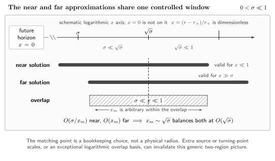
Schematic logarithmic validity map for $0<\sigma\ll1$, not to scale. The horizon $x=0$ is shown separately because it is not a point on the logarithmic axis. The near expansion is controlled for $x\ll1$, the far expansion for $x\gg\sigma$, and only the hatched interval $\sigma\ll x\ll1$ supports matching. Choosing $x_m\sim\sqrt{\sigma}$ balances the typical remainders $O(\sigma/x_m)$ and $O(x_m)$ at $O(\sqrt{\sigma})$; it does not identify a physical scale. Additional source or turning-point scales, or an exceptional logarithmic overlap basis, can invalidate this generic picture.

The same validity data in nonvisual form are:

Approximation	Quantity retained in its defining limit	Controlled region	Typical overlap remainder
Near	$X=x/\sigma$ at fixed $\overline\omega=W/2$	$x\ll1$	$O(\sigma/x)$
Far	$x$ after setting $\sigma=0$ at leading order	$x\gg\sigma$	$O(x)$
Common description	Both overlap expansions	$\sigma\ll x\ll1$	$O(\sigma/x_m)+O(x_m)$ at a chosen $x_m$

A scalar connection calculation

Use a massless scalar with the raw radial field $R$ defined by $\Psi=e^{-i\omega t+im\phi}S_{\ell m}(\theta)R(r)$. There is no spin-dependent horizon prefactor in this definition. The canonical scalar wave variable used elsewhere is $\sqrt{r^2+a^2}\,R$, not $R$ itself. Choose $m\gt0$, fixed $(\ell,m)$, and abbreviate $q=\overline\omega$. Set

$$\begin{aligned} K&=A_{0\ell m}(m/2)+m^2/4,\\ h&=\frac12+\sqrt{\frac14+K-2m^2}. \end{aligned}$$

The square root has nonnegative real part and positive imaginary part for a negative radicand. For the generic formulas below assume $2h-1\notin\mathbb Z$ and no singular denominator parameter. Initially $\operatorname{Im}q\gt0$ fixes retarded continuation; a real nonzero $q$ is its boundary value. The calculation gives leading small-$\sigma$ connection data, not a uniform spectral error theorem.

To see what is being expanded, write the exact scalar radial equation as

$$\begin{aligned} \bar a&=\frac a{r_+}=\sqrt{1-\sigma},\qquad k=\omega r_+=\frac{m\sqrt{1-\sigma}+q\sigma}{2-\sigma},\\ \mathcal N(x)&=k[(1+x)^2+\bar a^2]-m\bar a =kx(x+2)+q\sigma,\\ 0&=\frac{d}{dx}\left[x(x+\sigma)\frac{dR}{dx}\right] +\left[\frac{\mathcal N(x)^2}{x(x+\sigma)} -\lambda_{0\ell m}(a\omega)\right]R. \end{aligned}$$

Here $\lambda_{0\ell m}=A_{0\ell m}+(a\omega)^2-2am\omega$, whose limit is $K-m^2$. These definitions are the scalar Teukolsky radial convention. They keep the horizon gap and detuning in the same numerator.

The near solution

At fixed $X=x/\sigma$ and $q$, the limiting equation is

$$\frac{d}{dX}\left[X(X+1)\frac{dR_{\mathrm N}}{dX}\right] +\left[\frac{(mX+q)^2}{X(X+1)}+m^2-K\right]R_{\mathrm N}=0.$$

The future-horizon branch has exponent $-iq$. Giving its $X^{-iq}$ coefficient the value one fixes

$$R_{\mathrm N}(X)=X^{-iq}(1+X)^{i(q-m)} {}_2F_1(h-im,1-h-im;1-2iq;-X).$$

Use real logarithms of $X$ and $1+X$ in the exterior. Hypergeometric continuation gives the two complete Frobenius series at $X\gg1$:

$$\begin{aligned} R_{\mathrm N}&=a_{\mathrm N}X^{h-1}[1+O(X^{-1})] +b_{\mathrm N}X^{-h}[1+O(X^{-1})],\\ a_{\mathrm N}&=\frac{\Gamma(1-2iq)\Gamma(2h-1)} {\Gamma(h-im)\Gamma(h+im-2iq)},\\ b_{\mathrm N}&=\frac{\Gamma(1-2iq)\Gamma(1-2h)} {\Gamma(1-h-im)\Gamma(1-h+im-2iq)}. \end{aligned}$$

This follows from the standard two-term connection, not a fit to only the larger power; its descendants can exceed the smaller branch. It is the scalar translation of Yang et al. 2013, “Spectrum bifurcation,” Eqs. (3.13)–(3.16), p. 8 (PDF), after $y=X/(1+X)$. See also NIST DLMF, § 15.8, Eq. (15.8.2). In the common $x$ basis,

$$A_{\mathrm N}=\sigma^{1-h}a_{\mathrm N},\qquad B_{\mathrm N}=\sigma^h b_{\mathrm N}.$$

A unit $x^{-iq}$ horizon coefficient instead multiplies this entire solution by $\sigma^{-iq}$. Such a normalization change cannot be applied to only one connection coefficient.

The far solution

At fixed $x$, the leading equation is

$$\frac{d}{dx}\left(x^2\frac{dR_{\mathrm F}}{dx}\right) +\left[\frac{m^2x^2}{4}+m^2x-h(h-1)\right]R_{\mathrm F}=0.$$

This is also the exact raw scalar equation at extremality and $\mu\omega=m/2$. A normalized mouth basis is

$$f_p(x)=x^{p-1}e^{-imx/2}{}_1F_1(p+im;2p;imx), \qquad p=h,\ 1-h.$$

Each basis element has coefficient one at its respective leading mouth power. Thus $R_{\mathrm F}=A_{\mathrm F}f_h+B_{\mathrm F}f_{1-h}$, and matching gives $A_{\mathrm F}=A_{\mathrm N}$, $B_{\mathrm F}=B_{\mathrm N}$ to the retained order.

The arbitrary matching point must disappear. If $x_m$ lies in the overlap, the neglected near correction is typically $O(\sigma/x_m)$ and the neglected far correction is $O(x_m)$. Moving $x_m$ changes the truncated answer only at those orders. The balanced choice $x_m\sim\sqrt{\sigma}$ makes both errors $O(\sqrt{\sigma})$; it does not create a physical scale. This is a schematic truncation estimate, not a uniform relative error bound on a vanishing or strongly suppressed coefficient. Dependence on $x_m$ at leading order diagnoses inconsistent normalization, missing powers, or a nonexistent overlap.

Connection coefficients and resonances

Choose the extremal tortoise constant by $r_*/\mu=x+2\log x-2/x$. The large-$x$ incoming/outgoing scalar fields have the leading forms

$$v_{\mathrm{in}}=x^{-1-im}e^{-imx/2},\qquad v_{\mathrm{out}}=x^{-1+im}e^{imx/2}.$$

The $x^{\pm im}$ factors are the long-range logarithmic phases, not optional amplitude powers. With $\operatorname{Log}(\pm im)=\log m\pm i\pi/2$, Kummer continuation gives

$$\begin{aligned} f_p&\sim I_pv_{\mathrm{in}}+O_pv_{\mathrm{out}},\\ I_p&=\frac{\Gamma(2p)}{\Gamma(p-im)}(-im)^{-p-im},\\ O_p&=\frac{\Gamma(2p)}{\Gamma(p+im)}(im)^{-p+im}. \end{aligned}$$

The complete connection, including both throat scale factors, is therefore

$$\begin{pmatrix}Z^{\mathrm{in}}\\ Z^{\mathrm{out}}\end{pmatrix} = \begin{pmatrix}I_h&I_{1-h}\\ O_h&O_{1-h}\end{pmatrix} \begin{pmatrix}\sigma^{1-h}a_{\mathrm N}\\ \sigma^h b_{\mathrm N}\end{pmatrix}.$$

These coefficients multiply $1/x$. At the limiting frequency the coefficients multiplying $1/r$ are $\mu Z^{\mathrm{in,out}}$; changing the tortoise additive constant also changes their phases. This is a scalar-field connection, not a gravitational flux conversion. The far basis and its outgoing condition agree with Yang et al. 2013, “Spectrum bifurcation,” Eqs. (3.7)–(3.9) and footnote 3, p. 7 (PDF).

Two checks test the normalization. First, with $W[f,g]=fg'-gf'$, $x^2W[f_h,f_{1-h}]=1-2h$ at the mouth, whereas $x^2W[v_{\mathrm{in}},v_{\mathrm{out}}]\to im$ at infinity. Gamma reflection gives the same determinant:

$$I_hO_{1-h}-I_{1-h}O_h=\frac{1-2h}{im}.$$

Second, match the field and its first derivative at any overlap point $x_m$. The coefficients agree:

$$A_{\mathrm F}=A_{\mathrm N},\qquad B_{\mathrm F}=B_{\mathrm N}.$$

The power-basis Wronskian is

$$W[x^{h-1},x^{-h}]_{x=x_m}=\frac{1-2h}{x_m^2}\ne0.$$

The arbitrary $x_m$ cancels from the coefficients.

A physical nonexceptional example can be specified without inventing an angular eigenvalue. For the lowest scalar branch $\ell=m=1$, the angular operator is the fixed-$m$ spherical operator plus $\sin^2\theta/4$. Positivity gives $K\gt2$, while the Rayleigh trial $S=\sin\theta$ gives $K\le2+1/5$: its weighted mean of $\sin^2\theta$ is $4/5$. Thus $1\lt2h-1\le\sqrt{9/5}\lt2$. Choosing, for example, $q=1/3$ yields the nonresonant connection above, with $K$ defined by the regular angular problem.

The approximate quasinormal condition is the combined $Z^{\mathrm{in}}=0$, not a pole of one Gamma factor. It retains the exterior coefficients, but does not certify an exact finite-$\sigma$ pole or nonzero excitation by given data. Nor is the critical-frequency far field a uniform phase approximation at arbitrarily large radius: a frequency error times unbounded $r_*$ need not be small. Keep the exact finite-$\sigma$ frequency in the radiation phases before taking the connection-coefficient limit.

For a sourced Green function the normalization is equally important. A horizon-normalized near solution can grow as a power of $\sigma$, while the amplitude excited by a fixed far-zone source contains the reciprocal or an additional suppression. Gralla, Zimmerman, and Zimmerman retain the far source, sum the near-horizon poles, and obtain a cross-region Green function with explicit dependence on $X=x/\sigma$ and $\sigma t$ Gralla, Zimmerman, and Zimmerman 2016, § II, pp. 2–4. This is why a local NHEK solution alone does not determine an observed waveform amplitude.

Exceptional frequencies and loss of uniformity

Three exceptions require a fresh expansion. First, when $2h-1$ is an integer, the two overlap powers become resonant and logarithms can replace one basis element. Gamma-function formulas that divided by their difference are then singular even if the exact solution is regular. Second, at special frequencies a nominal leading coefficient can vanish; a subleading near or far term then becomes leading. A pole in one gamma factor may also be canceled by a zero in another or by the Green-function numerator.

The simplest explicit test is $h=1/2$, where the two powers shown above coincide. Take the full limiting solution, not its separately divergent Gamma coefficients. Write its finite near logarithmic coefficients as $a_{\log},b_{\log}$. A valid raw-scalar overlap basis is then

$$\begin{aligned} R_{\mathrm N}&\sim X^{-1/2} \left[a_{\log}+b_{\log}\log X\right],\\ R_{\mathrm F}&\sim x^{-1/2} \left[A_{\log}+B_{\log}\log x\right]. \end{aligned}$$

Matching the constant and logarithmic terms gives

$$B_{\log}=\sigma^{1/2}b_{\log},\qquad A_{\log}=\sigma^{1/2}(a_{\log}-b_{\log}\log\sigma).$$

Equivalently, absorb $\sigma^{1/2}$ into finite near coefficients in the common $x$ basis: then $B_{\mathrm F}=B_{\mathrm N}$ and $A_{\mathrm F}=A_{\mathrm N}-B_{\mathrm N}\log\sigma$. These finite logarithmic coefficients are not the individual generic Gamma coefficients before the limit. No arbitrary matching radius appears. A pole obtained by dividing a generic connection formula by $2h-1$ at this point is therefore a basis failure, not by itself a physical resonance. The finite logarithmic coefficient is the quantity that must be compared with the limiting exact solution.

Third, the synchronous point cannot be reached by setting $\omega=m\Omega_H$ inside a formula derived at fixed nonzero $\overline\omega$ without checking uniformity. In the finite-temperature near equation above, $q=0$ makes the two horizon exponents $\pm iq$ coalesce; the regular singular points remain $X=0,-1,\infty$. This differs from the strict NHEK Whittaker equation at $\widehat\omega=0$, where the irregular horizon terms disappear. Similarly, $\sigma\to0$ at fixed exterior $\omega-m\Omega_H$ sends $\overline\omega\to\infty$ and exits the assumed matching regime.

The order of the near-zone and observation limits matters as well. At fixed $x>0$, the region $x=O(\sigma)$ collapses onto the horizon. Holding $X=x/\sigma$ fixed instead follows a throat observer. A response large in transverse derivatives for one observer may occupy a vanishing radial layer for the other. This nonuniformity can produce transient amplification; it does not change a lower-half-plane quasinormal pole into an exponentially growing mode.

The two spectral branches are compared in Zero-Damped and Damped Mode Families. The horizon consequence of the same scaling is developed in Aretakis Growth and Near-Extremal Transients.

Exercises

Suppose two approximations to the same raw radial field have leading overlap forms, with distinct toy exponents $p_1,p_2$,

$$R_{\mathrm N}=Ax^{p_1}+Bx^{p_2} +O\!\left(\frac{\sigma}{x}\right), \qquad R_{\mathrm F}=Cx^{p_1}+Dx^{p_2}+O(x).$$

Assume the displayed error orders also hold after $x\partial_x$. Show why the leading connection is independent of a matching point $x_m$, and estimate the best error obtained by balancing the two remainders.

Solution

Matching the value and first derivative at any $\sigma\ll x_m\ll1$ gives two independent linear equations. Because $x_m^{p_1}$ and $x_m^{p_2}$ have nonzero Wronskian when $p_1\ne p_2$, their leading coefficients must agree:

$$C=A,\qquad D=B.$$

No $x_m$ appears in this leading result. The mismatch is bounded schematically by

$$\mathcal E(x_m) =O\!\left(\frac{\sigma}{x_m}\right)+O(x_m).$$

Choosing $x_m\sim\sqrt{\sigma}$ balances the terms and gives $\mathcal E=O(\sqrt{\sigma})$ as a common-field and weighted-derivative truncation indicator, not a uniform relative error in either coefficient. If $p_1=p_2$, the basis loses independence and a logarithmic solution must be constructed; the preceding matching equations cannot simply be divided by $p_1-p_2$.

References

• Gralla, S. E., Zimmerman, A., and Zimmerman, P. (2016). “Transient instability of rapidly rotating black holes.” Physical Review D 94, 084017. DOI.
• National Institute of Standards and Technology. n.d. Digital Library of Mathematical Functions. § 15.8, transformations of the hypergeometric function, Eq. (15.8.2). Online reference.
• Yang, H., Zhang, F., Zimmerman, A., Nichols, D. A., Berti, E., and Chen, Y. (2013). “Branching of quasinormal modes for nearly extremal Kerr black holes.” Physical Review D 87, 041502(R). DOI.
• Yang, H., Zimmerman, A., Zenginoğlu, A., Zhang, F., Berti, E., and Chen, Y. (2013). “Quasinormal modes of nearly extremal Kerr spacetimes: Spectrum bifurcation and power-law ringdown.” Physical Review D 88, 044047. DOI.