Radiation Moments and Closure

Scrollable formula. Use Left and Right arrow keys to reveal hidden content.

Scrollable table. Use Left and Right arrow keys to reveal additional columns.

Scrollable figure. Use Left and Right arrow keys to inspect hidden content.

Radiation moments replace an angle-dependent distribution by energy density, flux, and a finite number of higher angular moments. Integrating the transfer equation gives exact evolution equations, but each moment couples to the next; a closure supplies the missing angular information. A useful closure must recover isotropic diffusion and directed free streaming, preserve realizability, and state what information it destroys. No algebraic two-moment closure can represent every multi-beam radiation field.

Required background. Hilbert Stress–Energy from Metric Variation supplies radiation stress and four-force exchange; Differential Equations supplies hyperbolic moments and diffusion limits.

Helpful background. The Einstein Equation supplies curved-spacetime coupling; Relativistic Matter and Compact Objects gives the transport hierarchy; and Computational Relativity supplies conservative evolution and stiff-source methods.

Energy, flux, and pressure moments

For an observer $u^a$ with projector $h^{ab}=g^{ab}+u^au^b$ , decompose the radiation stress tensor as

R^{ab}=E u^au^b+2u^{(a}F^{b)}+P^{ab},

where $F^au_a=0$ and $P^{ab}u_b=0$ . In the observer’s orthonormal frame, let $I(\boldsymbol\ell)=\int_0^\infty I_\nu(\boldsymbol\ell)\,d\nu$ be frequency-integrated intensity and $\ell^i$ a unit propagation direction. Then

E=\int I\,d\Omega,\qquad F^i=\int I\ell^i\,d\Omega,\qquad P^{ij}=\int I\ell^i\ell^j\,d\Omega.

These are respectively the angular zeroth, first, and second moments. The absence of explicit $c$ factors follows from the inherited $c=1$ units. For nonnegative intensity,

P^a{}_a=E, \qquad F_aF^a\leq E^2.

The trace identity follows from $\ell_i\ell^i=1$ . The flux bound follows from $|\int I\boldsymbol\ell\,d\Omega|\leq\int I\,d\Omega$ ; equality requires all occupied directions to coincide. These are necessary realizability conditions: a candidate pressure tensor must also be positive semidefinite and compatible with the lower moments. Matter exchange is described by a four-force $G^a$ ,

\nabla_aR^{ab}=-G^b, \qquad \nabla_aT_{\rm matter}^{ab}=G^b.

For a fixed inertial observer in flat spacetime, the projections are particularly transparent:

\partial_tE+\partial_iF^i=-G^0, \qquad \partial_tF^i+\partial_jP^{ij}=-G^i.

Four equations evolve $E$ and the three components of $F^i$ , but the pressure tensor remains unknown. Specifying $P^{ij}(E,F)$ closes this system by choosing an angular model. The covariant moment construction and frame transformations are given in Foucart 2023, §§ 4.2.1–4.2.2.

Diffusion, streaming, and M1 closure

In an optically thick medium the distribution is nearly isotropic in the material frame. For a stationary, homogeneous material background in flat spacetime, neglecting the flux time derivative relative to scattering relaxation gives

P^{ab}\to\frac{E}{3}h^{ab}, \qquad F^a\simeq-\frac{1}{3\kappa}\,h^{ab}\nabla_bE,

where $\kappa$ is the transport opacity in inverse-length units. Indeed, $G^i=\kappa F^i$ and $P^{ij}\simeq E\delta^{ij}/3$ in the local moment equation give this result. It is a local diffusion approximation, not the full covariant flux law for accelerating or shearing matter; general observer projections include acceleration and velocity-gradient terms. In vacuum a single beam with unit spatial direction $n^a$ has

F^a=E n^a, \qquad P^{ab}=E n^an^b.

For $E\gt0$ , M1 interpolates algebraically using the reduced flux $f=\sqrt{F_aF^a}/E$ . The empty state $E=0$ requires $F^a=P^{ab}=0$ and is handled separately. For $F^a\neq0$ , let $n^a=F^a/|F|$ and write

P^{ab}=E\left[ \frac{1-\chi}{2}h^{ab} +\frac{3\chi-1}{2}n^an^b \right].

The Levermore choice

\chi(f)=\frac{3+4f^2}{5+2\sqrt{4-3f^2}}

gives $\chi(0)=1/3$ and $\chi(1)=1$ . At $F=0$ , the direction $n^a$ is undefined, but its coefficient vanishes and the tensor has the unique isotropic limit. The formula is reproduced, with its distinct derivation separated from other entropy closures, in Mezzacappa et al. 2020, § 4.7.4, Eq. (143).

For grey massless radiation, this particular closure can be understood without an entropy argument: assume the radiation is isotropic in some radiation rest frame, where $R^{ab}=\operatorname{diag}(E_0,E_0/3,E_0/3,E_0/3)$ . A Lorentz boost of speed $\beta$ along $x$ gives

E=\frac{E_0(3+\beta^2)}{3(1-\beta^2)},\qquad F^x=\frac{4E_0\beta}{3(1-\beta^2)},\qquad P^{xx}=\frac{E_0(1+3\beta^2)}{3(1-\beta^2)}.

Consequently $f=4|\beta|/(3+\beta^2)$ and $\chi=(1+3\beta^2)/(3+\beta^2)$ ; eliminating $\beta$ gives the displayed Levermore function. This explains both its realizability and its restriction: a general radiation field need not be a boosted isotropic distribution. Neither this algebraic closure nor a numerical discretization automatically enforces the Pauli bound for energy-dependent fermion occupations.

Flux-limited diffusion instead evolves primarily $E$ and modifies the diffusion coefficient so $|F|\leq E$ . It is efficient in thick regions but does not retain a genuinely hyperbolic free-streaming flux equation. The two approaches can agree asymptotically yet differ substantially near transparent, time-dependent, or multi-directional regions.

The crossing-beam counterexample

Take two equal, noninteracting beams traveling along $+x$ and $-x$ . With $\delta_\Omega$ normalized to unit integral on the sphere, their intensity is

I(\boldsymbol\ell)=\frac E2\left[ \delta_\Omega(\boldsymbol\ell-\hat{\boldsymbol x}) +\delta_\Omega(\boldsymbol\ell+\hat{\boldsymbol x})\right].

The first angular moment is odd under $\boldsymbol\ell\mapsto-\boldsymbol\ell$ , so the fluxes cancel,

F^x=0,

but their pressures add,

P^{xx}=E, \qquad P^{yy}=P^{zz}=0.

Any algebraic M1 closure sees only $E$ and $F=0$ , interprets the field as isotropic, and returns $P^{ij}=E\delta^{ij}/3$ . It cannot know that two beams crossed. In two spatial dimensions, crossing non-opposed beams can instead merge into an artificial beam. This is an information limit of the retained moments, not a bug repaired by grid refinement.

An isotropic field $I=E/(4\pi)$ has the same $E$ and $F=0$ but pressure $E\delta^{ij}/3$ , because rotational symmetry gives $\int\ell^i\ell^j\,d\Omega=(4\pi/3)\delta^{ij}$ . The two different second moments cannot both be reconstructed from identical lower moments. Foucart discusses closure limits in Foucart 2023, §§ 4.2.5 and 4.2.9. A hybrid method can use higher angular resolution or Monte Carlo packets where multi-beam structure matters, but its coupling must conserve total energy and momentum.

Compare the pressure tensors in the figure: zero net flux can mean either cancellation of two directed beams or cancellation among every direction. The lower moments do not distinguish these possibilities.

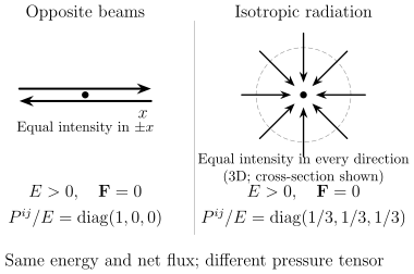
Equal opposed beams and an isotropic radiation field have the same energy and zero flux, but the beams have pressure only along their axis while isotropic radiation has one third of the energy in each diagonal pressure. — Identical energy $E$ and net flux $\mathbf F=0$ do not determine the pressure tensor. Opposed beams give $P^{ij}/E=\operatorname{diag}(1,0,0)$ ; isotropic radiation gives $P^{ij}/E=\operatorname{diag}(1/3,1/3,1/3)$ . The angular drawings are schematic; the isotropic panel is a cross-section of a three-dimensional field. The displayed moment relations are exact.

Benchmark suite and documented environment

The continuum inputs are the grey two-moment balance equations, a specified closure, opacity field, initial $E$ and $F$ , and boundary conditions. Four complementary benchmarks are needed:

a vacuum pulse with $F^x=E$ , which should translate at unit speed without violating $|F|\leq E$ ;
a homogeneous isotropic state with $F=0$ , which should remain stationary;
an optically thick Gaussian energy perturbation, whose late-time width follows diffusion coefficient $D=1/(3\kappa)$ ;
two crossing beams, used to document rather than conceal the M1 failure.

A possible numerical experiment uses binary64 arithmetic, finite volumes, a declared approximate Riemann flux, second-order reconstruction, and an implicit–explicit treatment of absorption and scattering sources. Record the executable, exact software versions, inputs, and output definitions when performing it. This page gives analytic reference states and a proposed numerical test, without claiming an executed transport calculation.

Use $N=64,128,256$ cells for one-dimensional tests and matched $64^2,128^2,256^2$ grids for crossing beams. Report $L_1$ errors against analytic free-streaming and diffusion solutions, observed order, maximum violation of $E\geq0$ and $|F|\leq E$ , total radiation-plus-matter energy error, and sensitivity to halving the Courant factor and source tolerance. In the thick test, refine the macroscopic gradient scale and diffusion evolution time while varying the cell optical depth independently. An asymptotic-preserving method should approach the diffusion limit even when the mean free path is smaller than a cell and the interaction time is shorter than a timestep; requiring both microscopic scales to be resolved would miss that property.

One failure mode is negative $E$ from reconstruction; others include superluminal reduced flux, excessive diffusion in vacuum, unstable explicit treatment when $\kappa\Delta t\gg1$ , incorrect equilibrium from inconsistent emissivity and absorption, and artificial beam collision from M1. The final item should persist with refinement and be labeled closure uncertainty rather than truncation error.

Exercises

Now let the two equal beams travel along $\boldsymbol\ell_\pm=(\cos\theta,\pm\sin\theta,0)$ , with $0\leq\theta\leq\pi/2$ . Find the exact flux and pressure. For $\theta=\pi/3$ , can an M1 closure about the net-flux axis recover that pressure?

Solution

Adding the two first and second moments gives

\frac{\mathbf F}{E}=(\cos\theta,0,0), \qquad \frac{P^{ij}}E=\operatorname{diag}(\cos^2\theta,\sin^2\theta,0).

For $\theta=\pi/3$ , $f=1/2$ and the exact diagonal pressures are $(1/4,3/4,0)E$ . M1 is axisymmetric about $x$ , so it must assign equal $y$ and $z$ pressures. Levermore M1 gives $\chi=(5-\sqrt{13})/3\simeq0.4648$ , hence diagonal pressures approximately $(0.4648,0.2676,0.2676)E$ . The discrepancy is present even when the input moments are exact.

References

Foucart, François. “Neutrino Transport in General Relativistic Neutron Star Merger Simulations.” Living Reviews in Computational Astrophysics 9, 1 (2023). DOI.
Mezzacappa, Anthony, Eirik Endeve, O. E. Bronson Messer, and Stephen W. Bruenn. “Physical, Numerical, and Computational Challenges of Modeling Neutrino Transport in Core-Collapse Supernovae.” Living Reviews in Computational Astrophysics 6, 4 (2020). DOI.