Adaptive Mesh Refinement

Adaptive mesh refinement concentrates resolution near horizons, stars, shocks, or propagating waves while leaving distant regions coarse. It also inserts new numerical operations—prolongation, restriction, subcycled time interpolation, synchronization, and regridding—that can dominate the error even when every uniform-grid stencil is high order. A trustworthy AMR calculation therefore tests interfaces with known waves and conserved quantities before relying on a physical simulation, and it varies refinement criteria rather than treating one hierarchy as exact.

Helpful background. Formulations of General Relativity supplies evolved fields and constraints, Ordinary Differential Equations supplies time stepping, Computational Relativity supplies common verification standards, and Probability and Statistical Inference supplies uncertainty comparisons across refinement policies.

The AMR operators

Nested grid refinement with ratio $r$ replaces a coarse cell size $H$ by $h=H/r$. Fine-grid ghost zones are filled by spatial prolongation and, under subcycling, temporal interpolation. Fine data are restricted back to the coarse level after synchronization. For conservative systems, refluxing corrects coarse cells with the difference between accumulated fine and coarse interface fluxes.

The implementation must record refinement ratios, time-subcycling schedule, prolongation and restriction orders, buffer width, regridding cadence, tagging criterion, nesting rules, and treatment of each tensor or conserved variable. Schnetter, Hawley, and Hawke 2004, §II.B and §IV, Figures 7–9 and 11–15 describes Berger–Oliger-style mesh refinement for numerical relativity and exposes interface considerations.

A high-order interior stencil loses its designed order if prolongation or time interpolation is lower order. Buffer zones must be wide enough that fine points used for an update do not depend on stale coarse data. Regridding creates or deletes degrees of freedom; preserve constraints and conserved integrals across that event and output the correction.

Why restriction does not replace refluxing

Consider $\partial_tU+\partial_xF=0$ on a fixed one-dimensional grid. Put an uncovered coarse cell of width $H$ immediately left of a ratio-two fine patch. Count interface flux as positive toward increasing $x$, from coarse to fine. Over one coarse step $\Delta t$, let the time-integrated fluxes per unit area be

$$I_c=\Delta t\,\overline F_c, \qquad I_f=\frac{\Delta t}{2} \left(\overline F_f^{(1)}+\overline F_f^{(2)}\right),$$

where each bar denotes the time average for that step, including all Runge–Kutta stage weights. The provisional coarse update loses $I_c$, while the fine patch gains $I_f$. Their combined conserved integral therefore acquires the spurious amount $I_f-I_c$. Refluxing corrects the adjacent uncovered coarse-cell average by

$$U_C\longleftarrow U_C-\frac{I_f-I_c}{H}.$$

For example, $H=1$, $I_c=0.10$, and $I_f=0.12$ require a coarse correction $-0.02$. Adding $+0.02$ doubles the conservation defect. In several dimensions use face-area-integrated fluxes and divide by coarse-cell volume. At synchronization, restriction instead replaces a covered coarse average by the volume-weighted average of its fine children. It does not correct the neighboring uncovered cell’s mismatched flux. These operations are the conservative synchronization mechanism of Berger and Colella 1989, §3, pp. 68–71.

The conserved integral is evaluated on the composite mesh: count fine cells inside refined patches and coarse cells only outside them. Counting both representations of the same region produces an apparent conservation error even when every flux is correct.

Follow one synchronization interval in the figure. The fine level needs data at intermediate times even though the coarse level has taken only one step. The upper transfer then corrects the coarse result with information from both fine steps.

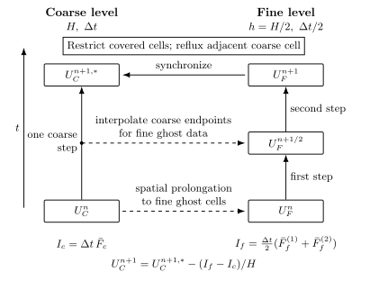
Ratio-two subcycling for a Cartesian conservative scheme, shown schematically. Intermediate ghost data interpolate the coarse endpoints; the midpoint dot is not an additional coarse step. Restriction replaces covered coarse values, while reflux replaces the adjacent uncovered cell’s provisional $U_C^{n+1,*}$ by the corrected $U_C^{n+1}$. Here that cell is left of the fine patch and positive interface flux points right. Barred fluxes include all time-integration stage weights. Not to scale.

Tag what controls the scientific error

Common indicators use gradients, truncation estimates from shadow hierarchies, constraint residuals, shock sensors, or geometric distances from compact objects. A threshold is a numerical parameter. Sweep it, cap level changes, and record hysteresis so repeated refinement–derefinement does not generate noise.

Tagging only a constraint can miss a smooth waveform phase error; tagging only density can underresolve magnetic or metric fields. Combine indicators according to the observable. Fixed moving boxes are predictable and inexpensive for orbiting compact objects but may waste cells or miss ejecta; fully dynamic tagging is flexible but introduces irregular load and regridding noise. Neither policy is universally superior.

Interface benchmarks

Use a complex periodic wave, or two real fields representing its real and imaginary parts, so leakage into an initially absent Fourier component can be measured unambiguously:

$$\partial_tq+\partial_xq=0, \qquad q_{\rm ex}(t,x)=e^{2\pi i(x-t)}.$$

The domain is $[0,1]^3$, all boundaries are periodic, and the initial data are $q(0,x)=e^{2\pi ix}$. Place a stationary ratio-two refined patch on $x\in[1/4,3/4]$ across the full transverse area, use fourth-order finite-volume reconstruction and transfers, conservative refluxing, factor-two subcycling, RK4, and CFL $0.2$. Run base grids $N^3$ with $N=32,64,128$ to $t=1$; a uniform grid at the corresponding fine spacing is a secondary reference, while $q_{\rm ex}$ is the primary analytic reference.

Compare cell averages with exact cell averages using the volume-weighted relative $L_2$ error $E_2$. Also record

$$A_{\rm opp}=\frac{|\hat q_{-1}|}{|\hat q_{+1}|}, \qquad C_q=\frac{\left|\int(q(t)-q(0))\,d^3x\right|} {\int|q(0)|\,d^3x},$$

where the Fourier coefficients and integrals are assembled independently on the composite mesh without double-counting covered coarse cells. Accept the $N=128$ hierarchy only if $E_2\leq10^{-5}$, $A_{\rm opp}\leq10^{-6}$, $C_q\leq10^{-12}$, and successive $E_2$ values approach fourth-order reduction. Repeat after shifting both fine interfaces by $1/16$ and after disabling subcycling; neither variation may change the finest $E_2$ by more than $20\%$. These are prospective acceptance limits, not measured outcomes.

Here $A_{\rm opp}$ measures spectral contamination, not a physically reflected left-moving wave: both positive and negative Fourier wave numbers of this one-way advection equation propagate to the right. To measure reflection as a propagation direction, also evolve a two-way wave system, for example $u_t=p$, $p_t=u_{xx}$, and separate its left- and right-going characteristic amplitudes.

For strong scaling, hold the complete $N=128$ hierarchy fixed and use $P/P_0=1,2,4,8$ resources. For weak scaling, tile $1,2,4,8$ identical periodic cubes, each with one $128^3$ base grid and the same refined patch, while assigning one tile per $P_0$ resources. Use one warm-up and seven measured repetitions, report median wall time and interquartile range, and include only layouts that satisfy the same $E_2$, $A_{\rm opp}$, and $C_q$ limits. The per-tile hierarchy must first pass the accuracy test; weak scaling does not make an under-resolved tile more accurate.

Observed discrepancy: not available—specification only.

For a source-free finite-volume conservation law with periodic boundaries, compatible refluxing should reduce the discrete global defect to accumulated roundoff, independently of the field’s truncation error. Physical sources, nonconservative repairs, and open-boundary fluxes need their own budget terms. For metric evolution, track constraints as a pulse crosses. Radia et al. 2022, §2.2, §3 and §§4–5, Figures 4–5 and 9 studies modern AMR infrastructure and strong-field tests relevant to these checks.

Then use a moving black hole or relativistic star with refinement boundaries crossing smooth exterior fields. Monitor horizon or stellar invariants, constraints, and spurious radiation. Sweep buffer size, regrid interval, tag thresholds, and prolongation order independently. A hierarchy that tracks the object perfectly can still reflect outgoing waves at every level transition.

The validity regime assumes that every dynamically important scale is covered by the maximum level and that coarse regions still resolve fields passed into fine boundaries. AMR cannot recover information already aliased on the base grid, and a maximum-level cap creates an unquantified limitation unless the tagged-but-unrefined region is reported.

Environment and failure criteria

Pin grid topology, ratios, level extents, subcycling, all transfer operators, refluxing, buffers, tagging and hysteresis, regrid cadence, load-balancing policy, base discretization, precision, and code revision. A clean interface could be amr-test --config crossing-pulse.toml --output run/, emitting hierarchy histories, interface fluxes, conserved integrals, reflections, constraints, refinement sweeps, and environment metadata. This specifies a rerun record and does not claim that code accompanied the page.

Reject an AMR result if interface reflections do not converge, conserved defects jump at synchronization, convergence order drops without an error budget, or the observable changes materially under a reasonable tagging sweep. Failure modes include stale ghost data, insufficient buffers, inconsistent tensor interpolation, regridding every step, and using the same under-resolved coarse base in every nominal refinement. Performance savings never compensate for a hierarchy-dependent scientific answer.

Diagnostic

A pulse converges at fourth order before crossing a level boundary and at second order afterward. Its integrated conserved quantity jumps at synchronization, while turning off subcycling removes the jump. Where is the likely defect?

Solution

The evidence points to temporal interpolation or coarse–fine synchronization, not the fourth-order interior stencil. Check fine ghost-zone time data, flux accumulation, refluxing, and buffer width. Refine the time interpolation, repeat with shifted interfaces and three scales, and require both the post-crossing waveform and conserved integral to recover their designed behavior.

References

• Berger, M. J., and Colella, P. (1989). “Local adaptive mesh refinement for shock hydrodynamics.” Journal of Computational Physics 82, 64–84. DOI.
• Radia, M., Sperhake, U., Drew, A., et al. (2022). “Lessons for adaptive mesh refinement in numerical relativity.” Classical and Quantum Gravity 39, 135006. arXiv.
• Schnetter, E., Hawley, S. H., and Hawke, I. (2004). “Evolutions in 3D numerical relativity using fixed mesh refinement.” Classical and Quantum Gravity 21, 1465–1488. arXiv.