Collocation and Relaxation Methods

Collocation solves a boundary-value problem as one coupled nonlinear system rather than integrating from one end. Unknown values or polynomial coefficients across the entire interval are adjusted until the differential equation and all boundary conditions are satisfied together. This avoids the directional instability of shooting, but introduces new obligations: residuals between collocation points, mesh adequacy, nonlinear branch selection, and matrix conditioning must all be measured.

Required background. Ordinary Differential Equations supplies boundary-value problems, interpolation, Newton iteration, and residuals.

Helpful background. Formulations of General Relativity provides relativistic systems that generate nonlinear radial equations, while Partial Differential Equations and Green Functions supplies separated boundary operators and elliptic intuition.

Global enforcement on a mesh

Write a first-order system as $y'=f(x,y,p)$ with boundary residual $g(y(a),y(b),p)=0$. A collocation method represents $y_h$ by piecewise polynomials and imposes the ODE at selected nodes,

$$r_h(x_j)=y_h'(x_j)-f(x_j,y_h(x_j),p)=0,$$

together with the boundary equations. Newton or a damped quasi-Newton iteration solves the resulting algebraic system. Relaxation is the same global idea expressed in finite-difference variables: update all mesh values at once from the linearized residual.

Because $r_h(x_j)=0$ by construction, the collocation-node residual is not an error estimate. Evaluate $r_h$ on an independent denser grid or integrate a residual norm. Adaptive schemes refine intervals whose defect exceeds a tolerance. Polynomial collocation and higher-order implementations are developed in Ascher, Mattheij, and Russell 1995, Chapter 5 § 5.4, pp. 218–225, and §§ 5.6.2–5.6.4, pp. 247–265; error estimation, adaptive meshes, linear solves, and nonlinear iteration in a concrete solver are described in Ascher, Christiansen, and Russell 1979, §§ 2–7, pp. 662–676.

Bratu’s two branches

Use the nonlinear benchmark

$$y''+\lambda e^y=0, \qquad y(0)=y(1)=0,$$

with $\lambda=1$. An analytic family is

$$y(x)=-2\log\!\left[ \frac{\cosh\bigl(\theta(x-\tfrac12)\bigr)}{\cosh(\theta/2)} \right], \qquad \lambda=\frac{2\theta^2}{\cosh^2(\theta/2)}.$$

Differentiating this expression gives $y''=-2\theta^2\operatorname{sech}^2[\theta(x-1/2)]$, while $e^y=\cosh^2(\theta/2)\operatorname{sech}^2[\theta(x-1/2)]$. The parameter relation therefore makes the differential residual vanish, and the evenness of $\cosh$ gives both boundary values. This verifies the family without relying on a solver.

For $\lambda=1$ the two positive roots are approximately $\theta=0.75858230$ and $5.46935139$. Their central values $y(1/2)=2\log\cosh(\theta/2)$ are approximately $0.14053921$ and $4.09146725$. Initialize the first-order state $(y,y')$ once with $(0,0)$ and once with $(16x(1-x),16(1-2x))$. These guesses distinguish the small and large solutions; a guess $4x(1-x)$ peaks at only one and can converge to the lower branch again. A guess is not a guarantee: identify the returned branch by its central value and compare with the exact family. Report the maximum solution error, independently sampled differential residual, boundary residual, Newton iterations, mesh size, and condition estimate. The two-solution test is also illustrated in the SciPy solve_bvp documentation, Examples, Bratu problem.

The branch is part of the input. A nonlinear solver that returns the lower branch from both guesses has not reproduced the upper solution, even if its residual is small. The fold follows from $d\lambda/d\theta=0$, or $\theta\tanh(\theta/2)=2$: it occurs at $\theta\simeq2.39935728$ and $\lambda\simeq3.51383072$. Ordinary continuation in $\lambda$ encounters a singular linearization there. Pseudo-arclength continuation instead augments the equations by a condition on distance along the solution curve, allowing the parameter to turn with the branch.

The figure makes the ambiguity visible: the line $\lambda=1$ intersects the solution curve twice. Follow those two points to the two profiles; both satisfy the same endpoint conditions.

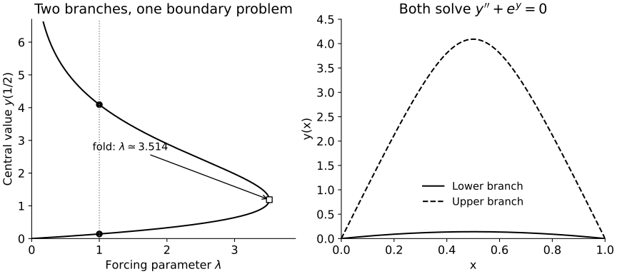
Exact dimensionless Bratu solutions for $y''+\lambda e^y=0$ with $y(0)=y(1)=0$. At $\lambda=1$, the central values are approximately $0.14054$ and $4.09147$; the branches meet at $\lambda\simeq3.51383$. These curves are evaluated from the analytic family, not fitted to solver output. Their labels make no claim about dynamical stability.

Refinement and independent comparison

Repeat both branches from uniform initial meshes with 5, 9, and 17 nodes at tolerances $10^{-6}$, $10^{-9}$, and $10^{-12}$, allowing at most 10,000 nodes. Evaluate residuals on a separate uniform 4001-point grid. Refine polynomial order and mesh spacing separately if the software permits it. Convergence requires decreasing solution error and off-grid residual on both branches. Repeat the finest case with at least 100-bit arithmetic to distinguish discretization error from a roundoff plateau.

Compare one branch with multiple shooting using the exact same boundary conditions and norm. Shooting and collocation have different numerical failure mechanisms, so agreement is useful. The directional sensitivity of shooting, against which the global solve is contrasted, is analyzed in Ascher, Mattheij, and Russell 1995, Chapter 3 § 3.4, pp. 110–126. An independent dense-grid substitution of the analytic solution supplies an additional benchmark that does not reuse either solver.

For problems on a compactified or singular domain, vary the domain map and endpoints. A residual weighted by the map Jacobian can hide endpoint contamination if only the computational coordinate is inspected. State which norm is physical and which is computational.

Environment and failure diagnostics

Pin the boundary-value library and version, interpolation degree, mesh-adaptation rule, nonlinear solver, Jacobian source, linear solver, arithmetic precision, tolerance definitions, maximum nodes, initial mesh, and initial guess. A clean rerun executes both Bratu branches, exports mesh and polynomial coefficients, evaluates an independent residual grid, and records refinement, precision, and initial-guess sweeps in machine-readable form.

The validity regime assumes a sufficiently smooth solution on each mesh interval and a nonsingular linearization away from the fold. Principal failure modes are maximum-node exhaustion, a singular Jacobian, damping stagnation, branch jumping, and a small node residual paired with a large between-node defect. Also reject apparent convergence when only the boundary residual improves, when the result changes substantially with a domain map, or when the adaptive mesh piles nodes at an unmodeled singularity.

Check your understanding

A Bratu run reports zero residual at every collocation node and satisfies both boundaries, but a dense independent grid finds a residual of $10^{-2}$ between nodes. Has the requested $10^{-8}$ tolerance been met?

Solution

No. The equations used to determine the polynomial vanish at the collocation nodes almost by definition. The off-grid defect shows that the polynomial or mesh is inadequate. Refine the mesh or order, repeat the independent residual norm, and verify convergence to the same analytic branch before accepting the solution.

References

• Ascher, U. M., Christiansen, J., and Russell, R. D. (1979), “A Collocation Solver for Mixed Order Systems of Boundary Value Problems,” Mathematics of Computation 33, 659–679. DOI.
• Ascher, U. M., Mattheij, R. M. M., and Russell, R. D. (1995), Numerical Solution of Boundary Value Problems for Ordinary Differential Equations, SIAM. DOI.
• SciPy developers (n.d.), “scipy.integrate.solve_bvp,” SciPy Reference Guide, Examples: Bratu problem. Documentation.

Further reading

• Virtanen, P., et al. (2020), “SciPy 1.0: Fundamental Algorithms for Scientific Computing in Python,” Nature Methods 17, 261–272. DOI.