From Scientific Question to Computational Experiment

A computational experiment is a finite attempt to answer a physical question: it fixes a mathematical model, turns that model into an algorithm, produces declared observables, and exposes enough controls that the result can fail. The central object is therefore not a code or a plot but a conditional claim—for these equations, data, conventions, numerical settings, and checks, this output approximates this quantity to this accuracy. This page develops that contract and tests it on a scalar-wave calculation simple enough to have an analytic answer.

Required background. Calculus and Linear Algebra for Relativity supplies norms, dimensional scaling, and conditioning; Differential Equations for Relativity supplies initial-value problems, stability, and error tolerances.

Helpful background. Formulations of General Relativity connects continuum formulations to their numerical realizations; Probability and Inference for Gravity supplies the language for ensembles and uncertainty.

The finite computational claim

Begin with a question narrow enough to be contradicted. “What happens in a binary-black-hole merger?” is a research program. “Does the dominant extracted strain mode change by less than $2\times10^{-3}$ in phase when the grid spacing and extraction radius are varied over the stated ranges?” is a computational question. It identifies an observable, a comparison, and a numerical scale.

A useful experiment record is the tuple

$$\mathcal E=(\mathcal M,\mathcal C,\mathcal I,\mathcal A,\mathcal N,\mathcal O,\mathcal V),$$

where $\mathcal M$ is the continuum model, $\mathcal C$ the conventions and units, $\mathcal I$ the initial and boundary data, $\mathcal A$ the algorithm, $\mathcal N$ the finite numerical controls, $\mathcal O$ the reported observables, and $\mathcal V$ the verification tests. Removing any entry changes what can be inferred. A waveform without its tetrad convention is ambiguous; a convergent sequence without a continuum target may converge to the wrong problem; an identical rerun without a physical benchmark may faithfully repeat an error.

The claim must also state its regime. Smooth-wave convergence does not establish shock-capturing accuracy. A vacuum test does not validate an equation-of-state table. Agreement before a reflected outer-boundary signal reaches the measurement region says nothing about later times. These restrictions belong beside the result, not in an implementation note.

This separation follows the standard distinction between obtaining a consistent computational result from the same inputs and testing a scientific conclusion through an independently designed study; the National Academies gives the definitions and their limitations in National Academies 2019, Summary pp. 6–8 and Chapter 3. The first is necessary evidence for a computational claim, but it is not the whole scientific case.

From field equation to executable specification

Consider a real massless scalar $u$ on $1+1$ dimensional Minkowski spacetime with the inherited signature $(-,+)$. On the periodic domain $x\in[0,2\pi)$ it obeys

$$-\partial_t^2u+\partial_x^2u=0, \qquad u(t,x)=\sin\!\bigl(k(x-t)\bigr),$$

with $k=2$. The exact right-moving solution fixes the initial data

$$u(0,x)=\sin(kx), \quad \Pi(0,x)=\partial_tu(0,x)=-k\cos(kx), \quad \Phi(0,x)=\partial_xu(0,x)=k\cos(kx).$$

Writing

$$\partial_tu=\Pi, \qquad \partial_t\Pi=\partial_x\Phi, \qquad \partial_t\Phi=\partial_x\Pi$$

gives a first-order system whose principal characteristic speeds are $0$ and $\pm1$. Its auxiliary constraint $\Phi-\partial_xu$ obeys $\partial_t(\Phi-\partial_xu)=0$, so an initial constraint error does not propagate away. A fourth-order centered derivative on a uniform grid is

$$(D_4 f)_j= \frac{-f_{j+2}+8f_{j+1}-8f_{j-1}+f_{j-2}}{12\,\Delta x},$$

with indices wrapped periodically. Pair it with classical fourth-order Runge–Kutta, a maximum Courant factor $\lambda_{\max}=1/4$, double precision, and resolutions $N=32,64,128,256$. To reach $T=1$ exactly with uniform steps, choose $m=\lceil T/(\lambda_{\max}\Delta x)\rceil$ and $\Delta t=T/m$; report the actual Courant factor $\Delta t/\Delta x$, which is at most $1/4$. These choices are part of the problem: changing the stencil, time step, precision, boundary treatment, or stopping time defines a different experiment.

The environment record should name the operating system or container digest, compiler and optimization flags or interpreter version, numerical-library versions, floating-point precision, source revision, thread and process counts, and relevant accelerator. The input record should serialize $k$, the domain, $N$, $\lambda$, final time, stencil, integrator, output cadence, and norm definitions in a stable key order. Its SHA-256 digest should be copied into every output record. A digest detects a changed byte; it does not establish that the byte encodes the intended equation.

A benchmark with an analytic discrepancy

For a Fourier mode $e^{ikx}$, the centered stencil has the exact modified wavenumber

$$\widetilde{k}= \frac{8\sin(k\Delta x)-\sin(2k\Delta x)}{6\,\Delta x} =k-\frac{k^5\Delta x^4}{30}+O(\Delta x^6).$$

The continuum initial data use $k$, not $\widetilde{k}$. Consequently they do not lie exactly on the discrete constraint surface: initially

$$\Phi-D_4u=(k-\widetilde{k})\cos(kx)=O(\Delta x^4).$$

This residual is constant under the semidiscrete equations. With $r_k=k/\widetilde{k}$, their exact semidiscrete solution for $u$ is therefore

$$u_h(t,x)=(1-r_k)\sin(kx)+r_k\sin(kx-\widetilde{k}t),$$

not a pure phase-shifted sine. This choice is deliberate: the same continuum initial field is sampled on every grid, the continuum energy remains exactly known, and the discrete constraint must converge at fourth order. If the root-mean-square error is

$$E_N(t)= \left[\frac{1}{N}\sum_{j=0}^{N-1} \bigl(u_j(t)-u(t,x_j)\bigr)^2\right]^{1/2},$$

then, before adding time-integration error,

$$\begin{aligned} E_N(1)=\frac{1}{\sqrt2}\Bigl(&[1-r_k+r_k\cos\widetilde{k}-\cos k]^2\\ &+[-r_k\sin\widetilde{k}+\sin k]^2\Bigr)^{1/2}. \end{aligned}$$

This relation is an independent analytic prediction, not a fit to numerical output. It gives the following reference values:

$N$	$\Delta x$	predicted $E_N(1)$
32	$1.9634954\times10^{-1}$	$9.8380638\times10^{-4}$
64	$9.8174770\times10^{-2}$	$6.2335419\times10^{-5}$
128	$4.9087385\times10^{-2}$	$3.9093779\times10^{-6}$
256	$2.4543693\times10^{-2}$	$2.4454640\times10^{-7}$

The observed order

$$p_N=\log_2\!\left(\frac{E_N}{E_{2N}}\right)$$

should approach four after temporal error and roundoff are smaller than spatial error. A useful predeclared acceptance rule is $3.8\lt p_N\lt4.2$ for the two finest pairs, $E_{256}\lt10^{-6}$, and agreement with the exact semidiscrete prediction to within the separately measured Runge–Kutta contribution. Halving $\Delta t$ at fixed $N$ isolates that contribution. The continuum energy

$$\mathscr H=\frac12\int_0^{2\pi}(\Pi^2+\Phi^2)\,dx=\pi k^2=4\pi$$

provides a conserved diagnostic in the declared Minkowski time slicing; at $N=256$, require relative drift below $10^{-7}$ for this short benchmark. The runnable example below measures these criteria rather than assuming them.

An independent check of the finite time step

The Runge–Kutta update for a scalar mode $v'=sv$ multiplies it by

$$R(z)=1+z+\frac{z^2}{2}+\frac{z^3}{6}+\frac{z^4}{24}, \qquad z=s\Delta t.$$

For the traveling part of this discrete wave, set $s=-i\widetilde k$ and $g=R(-i\widetilde k\Delta t)^m$. At the final time the fully discrete fields are therefore

$$\begin{aligned} u_j&=(1-r_k)\sin(kx_j)+r_k\operatorname{Im}(e^{ikx_j}g),\\ \Pi_j&=-k\operatorname{Re}(e^{ikx_j}g),\qquad \Phi_j=k\operatorname{Re}(e^{ikx_j}g). \end{aligned}$$

This formula uses a single complex amplification factor, independently of the real-space stencil loop. Agreement with it tests the discrete implementation. Agreement with the continuum wave tests the combined numerical error. Neither comparison should be substituted for the other.

The figure separates the total error from $\|u_{\Delta t}-u_h\|_{\mathrm{RMS}}$, the error caused by time stepping at fixed spatial discretization. Both decrease at fourth order here, so the slope alone cannot identify which error dominates; their magnitudes do.

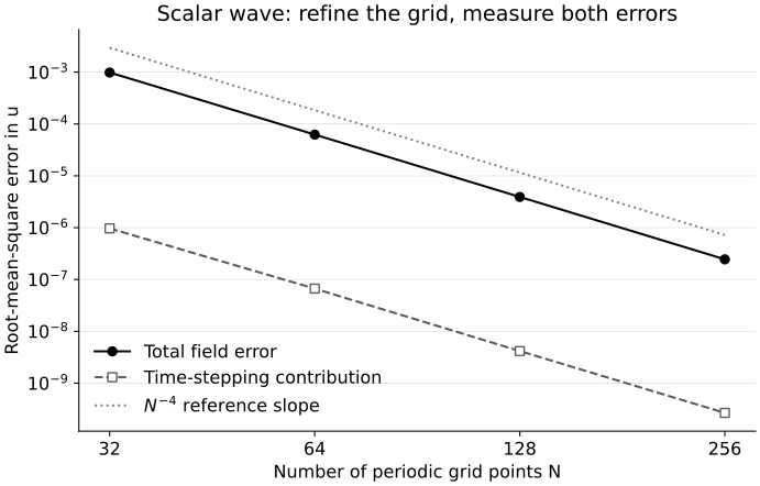
Measured RMS errors for the periodic $k=2$ wave at $T=1$, with fourth-order centered spatial differences and classical RK4 at maximum Courant factor $1/4$. Time stepping remains subdominant. The dotted $N^{-4}$ line is a reference slope, not an uncertainty bound; line segments only connect the four computed resolutions.

Precisely specified, portable testbeds have long been used to distinguish formulation or implementation failures from differences in the physical problem; representative numerical-relativity tests and their diagnostics are given in Alcubierre et al. 2004, §§ II–V. A single successful wave test remains narrow evidence: it does not exercise curvature, Einstein constraints, mesh refinement, shocks, excision, or long-time boundary contamination.

Controls that can falsify the result

Several checks answer different questions and should not be collapsed into one “validation” curve.

• Resolution refinement: does the solution approach a limit at the designed order while the physical setup is held fixed?
• Tolerance refinement: at fixed spatial resolution, do tighter nonlinear, linear, or time-integration tolerances stop changing the observable?
• Residual and constraint checks: does the computed field satisfy an independently evaluated differential equation or auxiliary constraint?
• Invariant or balance checks: are conserved energy, flux balance, symmetry, or a known zero maintained to the predicted accuracy?
• Boundary checks: does moving the outer boundary or changing a mathematically compatible boundary implementation leave the claimed time window unchanged?
• Independent calculation: does another discretization, analytic limit, manufactured solution, or separately implemented diagnostic reproduce the relevant quantity?

Agreement between two resolutions is not convergence if both are outside the asymptotic regime. A small residual is not sufficient if the residual is evaluated with the same faulty operator that produced the solution. Bitwise identity across two runs tests determinism, not physical correctness. Conversely, bitwise differences from parallel reductions need not be scientifically important when the observable agrees within a justified tolerance and the variation is measured over repeated runs.

The workflow should therefore preserve the raw per-resolution outputs, not only a final plot. It should also preserve the script or declarative rule that derives the table and figure from those outputs. The practical rules in Sandve et al. 2013, pp. 1–4, Rules 1–10 emphasize recording every transformation and retaining intermediate results; for numerical relativity, the additional requirement is that the transformations carry physical conventions and numerical error estimates with them.

Run the wave experiment

Download the scalar-wave program, its reference results, and the MIT license. The program uses Node.js 24.18.0 and only its standard library. Save the files together in an empty directory; no site checkout, package installation, network access or numerical library is needed. Run:

node scalar-wave.mjs > result.json
node scalar-wave.mjs --fields > result-with-fields.json

The first command recomputes all four grids and their half-time-step partners. The second additionally saves final arrays $x,u,\Pi,\Phi$. Both record the exact input specification, input and source SHA-256 digests, runtime, operating system, processor, actual time steps, errors and acceptance tests. The computation is serial and reads no cached results. A failed numerical criterion returns a nonzero exit status.

The retained binary64 run gives:

$N$	steps to $T=1$	total RMS error	temporal RMS contribution	order to next grid
32	21	$9.8433309\times10^{-4}$	$9.6646238\times10^{-7}$	3.98013
64	41	$6.2373966\times10^{-5}$	$6.6714829\times10^{-8}$	3.99502
128	82	$3.9118564\times10^{-6}$	$4.1705217\times10^{-9}$	3.99872
256	163	$2.4470731\times10^{-7}$	$2.6711765\times10^{-10}$	—

The largest fieldwise RMS discrepancy from the independent finite-step modal formula is below $3\times10^{-14}$ in this run. At $N=256$, relative energy drift is $7.73\times10^{-12}$. Comparing full and half steps with the semidiscrete field gives temporal orders between $3.9999$ and $4.0001$. The discrete constraint is preserved to a maximum RMS change below $1.4\times10^{-14}$, although its nonzero initial value still contributes to the continuum error. The stored JSON contains unrounded values and thresholds; other supported machines should be judged by those numerical tolerances, not by identical environment records or last bits.

Now make the calculation fail deliberately:

node scalar-wave.mjs --mutation=reverse-pi > wrong-sign.json

This changes $\partial_t\Pi=\partial_x\Phi$ to the opposite sign while retaining the original wave as the test target. It must return exit status 1 and failed checks, including the independent modal comparison. Inspect the changed error and energy, rather than merely noticing the nonzero exit status. Finally repeat the unmodified program in a second clean directory and compare the numerical rows. The reported run was also checked against an independent 80-decimal-digit evaluation of the semidiscrete errors.

The auxiliary constraint alone cannot diagnose this wrong sign: $\partial_t(\Phi-D_hu)=D_h\Pi-D_h\Pi=0$ still holds because neither of those two evolution equations was changed. Agreement with an independently known solution tests information that this constraint does not contain. At fine resolution the wrong-sign system also amplifies roundoff rapidly, so an eventual constraint failure is not its clean mathematical signature.

This is a small implementation-verification example. It does not supply the multi-thread, reduced-precision, stochastic-ensemble or archival-deposit experiments described on later pages, and it does not establish accuracy for curved spacetimes, shocks or physical outer boundaries.

The stopping rule is set before looking at the finest result: stop successfully only when the two finest refinement ratios are asymptotic, the temporal contribution is subdominant, the invariant and constraint thresholds pass, and the clean rerun agrees at the declared level. Stop unsuccessfully when a criterion fails. Adding resolutions after seeing an inconvenient answer is legitimate exploration, but the revised claim and rule must be recorded as a new experiment.

Common failure modes are hidden normalization changes, stale intermediate files, undeclared compiler or precision changes, output that silently overwrites its inputs, nondeterministic reductions treated as exact, and a workflow that cannot be started outside its creator’s directory. FAIR metadata can make data findable and reusable, but it does not alone show that a computation can be rerun; that distinction is explicit in Wilkinson et al. 2016, Box 2 and § “The principles precede implementation”.

Check your understanding

Two independently compiled programs use the same evolution routine and produce wave errors that agree to twelve digits at $N=128$. Both use an outer boundary whose reflected signal reaches the measurement point before the reported time. Does their agreement support the intended outgoing-wave claim?

Solution

No. The agreement supports reproducibility of the implemented, boundary-contaminated problem. Because both programs share the same algorithm and causal contamination, compilation independence is not a scientifically independent check. Move the boundary far enough that its domain of dependence cannot reach the measurement region, or impose and test a suitable absorbing condition; then repeat the resolution and boundary-location studies over the uncontaminated time interval.

References

• Alcubierre, Miguel, et al. “Toward Standard Testbeds for Numerical Relativity.” Classical and Quantum Gravity 21 (2004): 589–613. arXiv:gr-qc/0305023. DOI.
• National Academies of Sciences, Engineering, and Medicine. Reproducibility and Replicability in Science. Washington, DC: National Academies Press, 2019. DOI.
• Sandve, Geir Kjetil, Anton Nekrutenko, James Taylor, and Eivind Hovig. “Ten Simple Rules for Reproducible Computational Research.” PLOS Computational Biology 9, no. 10 (2013): e1003285. DOI.
• Wilkinson, Mark D., et al. “The FAIR Guiding Principles for Scientific Data Management and Stewardship.” Scientific Data 3 (2016): 160018. DOI.