Particle Horizons, Event Horizons, and Hubble Radius

Cosmology uses several lengths that can coincide in special solutions but answer different questions. Particle and event horizons are integrals over the past or future expansion history. The Hubble radius is an instantaneous expansion scale. A sound horizon depends on the propagation speed of a particular medium, and an apparent horizon is a quasi-local geometric surface. This page defines and evaluates each scale in idealized backgrounds; it does not address instrument calibration or current distance-ladder results.

Required background. Affine and Variational Geodesics supplies the Geodesics and Jacobi Fields capability used to integrate radial null curves and interpret causal reach.

Helpful background. The Einstein Equation supplies the Einstein Equations behind a specified $a(t)$; Relativistic Matter and Compact Objects supplies the Relativistic Matter and Compact Objects sound speeds used by material signals; Relativistic Cosmology orients the FLRW conventions; and The Wave Equation and Characteristics supplies the Waves, Green Functions, and Geometric Optics distinction between null and material characteristics.

Integral causal scales

For a radial FLRW null ray,

$$d\chi=\pm\frac{dt}{a(t)}.$$

Let $t_i$ denote the past endpoint of the cosmological history under consideration and $t_f$ its future endpoint. The comoving particle-horizon radius at time $t$ is

$$\boxed{ \chi_{\rm p}(t) =\int_{t_i}^{t}\frac{dt'}{a(t')} }, \qquad d_{\rm p}(t)=a(t)\chi_{\rm p}(t).$$

If this integral is finite, it gives a finite conformal reach. In a noncompact FLRW slice—or whenever the observer domain extends beyond that reach—a comoving observer at $t$ could not yet have received a signal from more distant points after $t_i$. In a compact or multiply connected slice, however, a finite reach may already cover or wrap around the whole spatial domain, so convergence alone does not guarantee a nontrivial particle horizon. If the integral diverges, that specified history has no finite particle horizon.

The comoving event-horizon radius is instead

$$\boxed{ \chi_{\rm e}(t) =\int_t^{t_f}\frac{dt'}{a(t')} }, \qquad d_{\rm e}(t)=a(t)\chi_{\rm e}(t).$$

It is finite only when the remaining future conformal time is finite. When the observer domain contains points beyond that reach, an inward-directed signal emitted there cannot ever reach the chosen comoving observer before $t_f$. Compact topology can instead let the finite reach cover the whole slice, so topology and observer domain remain part of the horizon statement. The definition depends on the entire future, so an event horizon cannot be inferred from $H(t)$ at one instant. Tong derives these null integrals and their convergence tests in Tong 2019, §1.1.4, printed pp. 15–19 (Official PDF).

The global causal and observer-domain qualifications are developed more fully in Observer, Acceleration, and Cosmological Horizons.

Local expansion and propagation scales

For $H\ne0$, define the physical Hubble radius and its comoving counterpart by

$$R_H=\frac{1}{|H|}, \qquad r_H=\frac{1}{a|H|}.$$

These use only local background data. They are not generally causal boundaries. On an expanding branch, the areal distance $R=a\chi$ of an incoming radial photon in a flat model obeys

$$\frac{dR}{dt}=HR-1.$$

At $R=H^{-1}$ the photon’s proper distance is instantaneously stationary. Outside it, that distance can initially grow even though the photon moves locally inward at light speed. If $H^{-1}$ later grows, the ray can cross it and reach the observer. This behavior makes the Hubble radius a useful dynamical scale, not a one-way causal barrier.

For a signal with physical propagation speed $c_s(t)$ relative to the comoving medium, the comoving sound horizon is

$$r_s(t) =\int_{t_i}^{t}\frac{c_s(t')\,dt'}{a(t')}.$$

It bounds causal communication by that mode under the assumed medium model. When $0\leq c_s\leq1$, it lies inside the particle horizon built from null signals. The shorthand “horizon crossing” $k=aH$ instead compares a comoving Fourier scale with the comoving Hubble scale; it is not automatically the crossing of a global horizon. Acoustic evolution is more naturally compared with $kr_s$.

For a constant propagation speed and an expanding power law $a=Ct^p$ with $C\gt0$ and $0\lt p\lt1$, the physical sound horizon is

$$d_s(t)=a(t)r_s(t)=\frac{c_st}{1-p}.$$

It is $2c_st$ in radiation domination and $3c_st$ in matter domination. A vacuum de Sitter background has no material sound horizon by itself: one must first supply a propagating medium or test field and its $c_s(t)$.

When $H^2+K/a^2\gt0$, FLRW has a marginal-sphere areal radius, conventionally called its apparent-horizon radius,

$$R_{\rm A} =\frac{1}{\sqrt{H^2+K/a^2}}.$$

To see the marginal condition, let $R=aS_K(\chi)$ be areal radius in the two-dimensional $(t,\chi)$ metric. Since

$$g^{AB}\partial_A R\,\partial_B R=0, \qquad [S_K'(\chi)]^2=1-KS_K^2(\chi),$$

the marginal sphere obeys $1-R^2(H^2+K/a^2)=0$. This gives the radius above. If $H^2+K/a^2=0$, there is no finite solution; if the combination is negative, there is no real solution at all. For example, Milne has $H^2+K/a^2=0$ and hence no finite apparent horizon despite its finite Hubble radius. On an expanding flat background the marginal expansion is the ingoing one: larger spheres have both future radial null expansions positive, so this surface should not be interpreted as a black-hole trapping boundary. Only in the spatially flat case does it equal $H^{-1}$ on an expanding branch; it still need not equal a particle or event horizon. Notice also that $d_{\rm p}=a\chi_{\rm p}$ and $d_{\rm e}=a\chi_{\rm e}$ are radial proper distances, whereas $R_{\rm A}$ is an areal radius when $K\ne0$.

Comparison axes

The useful comparison is not merely numerical size. The decisive axes are which part of the history is required, which signal or geometric structure is used, and whether the result is a global causal boundary.

Scale	Required information	Propagation or geometry	Global causal boundary?
Particle horizon	Past integral from $t_i$	Null signals	When finite reach leaves part of the observer domain inaccessible
Event horizon	Future integral to $t_f$	Null signals	When finite reach leaves part of the observer domain inaccessible
Hubble radius	Instantaneous $H(t)$	Local expansion	No, in general
Sound horizon	Past integral and $c_s(t)$	A specified material mode	Only for that mode and model
Apparent horizon	$a$, $H$, $K$, and a foliation	Marginal null expansion	Quasi-local, not an event horizon

Two entries may agree in one solution while remaining conceptually distinct because their information requirements differ.

Power-law and de Sitter checks

Take the expanding family $a(t)=Ct^p$ with $C\gt0$, $p\gt0$, $t\gt0$, $t_i=0$, and $t_f=\infty$. For $p\lt1$,

$$d_{\rm p}(t)=\frac{t}{1-p}, \qquad \chi_{\rm e}=\infty,$$

so a particle horizon exists but an event horizon does not. Radiation $(p=1/2)$ gives $d_{\rm p}=2t=H^{-1}$; matter $(p=2/3)$ gives $d_{\rm p}=3t=2H^{-1}$. The radiation equality is therefore accidental, not a definition.

For $p\gt1$, the particle integral diverges at the stated past endpoint while the event horizon is finite:

$$d_{\rm e}(t)=\frac{t}{p-1}, \qquad R_H=\frac{t}{p}.$$

The two scales are unequal for every finite $p\gt1$. At $p=1$, both relevant integrals diverge logarithmically. The Milne model is the especially sharp counterexample: it is the future-cone patch of Minkowski spacetime in expanding coordinates, has $H^{-1}=t$, and has neither a particle nor an event horizon for the full $t\gt0$ Milne history.

Flat de Sitter expansion, $a=e^{Ht}$ with constant $H\gt0$, has

$$d_{\rm e} =a(t)\int_t^\infty e^{-Ht'}dt' =H^{-1}.$$

Here the event and Hubble radii coincide. The particle horizon depends on the chosen past endpoint: a finite start gives $d_{\rm p}=H^{-1}[e^{H(t-t_i)}-1]$, while the idealized extension $t_i\to-\infty$ has no finite particle horizon in this flat patch.

Reading the conformal diagrams

The figure compares matter expansion with accelerated power-law expansion. Follow the solid incoming light rays: each crosses the dotted Hubble scale and reaches the observer. The gray horizon lines instead depend on whether the past or future conformal endpoint is finite.

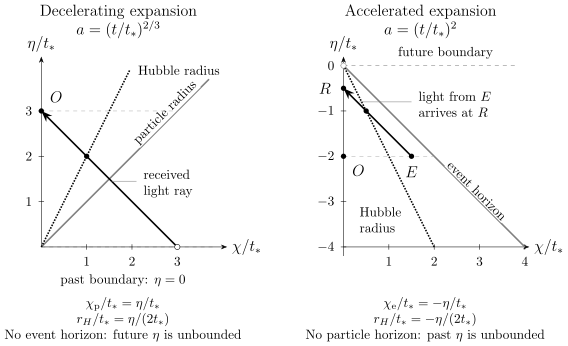
Incoming light crosses the dotted comoving Hubble radius $r_H=(aH)^{-1}$ and arrives. Left: $a=(t/t_*)^{2/3}$ has a finite past conformal endpoint and a particle horizon. Right: $a=(t/t_*)^2$ has a finite future conformal endpoint and an event horizon; light emitted at $E$ reaches $R$ after the time marked $O$. Here $t_*\gt0$, $0\lt t\lt\infty$, and the spatial slices are flat and noncompact. The axes use equal conformal-coordinate scales, not proper distances; angular directions are suppressed. The left ray’s open endpoint at $\eta=0$ is its limiting extrapolation to the excluded big-bang boundary.

The conformal origins are chosen so that the finite endpoint is at $\eta=0$. The same information can be read without the diagram:

Model	Conformal time	Particle radius	Event radius	Comoving Hubble radius
Matter	$\eta=3t_*(t/t_*)^{1/3}\gt0$	$\chi_{\rm p}=\eta$	No finite horizon	$r_H=\eta/2$
Accelerated power law	$\eta=-t_*(t/t_*)^{-1}\lt0$	No finite horizon	$\chi_{\rm e}=-\eta$	$r_H=-\eta/2$

In the right panel, at $\eta=-2t_*$ the emitter has $r_H=t_*\lt\chi_E=1.5t_*\lt\chi_{\rm e}=2t_*$. Its inward null ray arrives at $\eta=-0.5t_*$, before the future boundary. Being outside the Hubble radius at emission has not prevented communication.

Common pitfalls

Calling $H^{-1}$ “the horizon.” It is local and instantaneous. A particle or event horizon is an integral whose convergence depends on an endpoint of the spacetime history.

Omitting the lower or upper limit. A horizon statement is incomplete until the past or future endpoint and any extension of the model are specified.

Using one signal speed for every sector. Null rays, acoustic modes, and diffusive or interacting species have different propagation laws. Their causal scales need not coincide.

Exercises

For the accelerated power law $a(t)=Ct^2$ on $0\lt t\lt\infty$, determine the particle horizon, event horizon, Hubble radius, and comoving Hubble radius. Explain which quantities are genuine causal boundaries.

Solution

The past integral $\int_0^t dt'/(Ct'^2)$ diverges, so this specified power-law history has no finite particle horizon. The future integral is

$$\chi_{\rm e}(t) =\int_t^\infty\frac{dt'}{Ct'^2} =\frac{1}{Ct},$$

and therefore

$$d_{\rm e}=a\chi_{\rm e}=t.$$

Since $H=2/t$,

$$R_H=\frac{t}{2}, \qquad r_H=\frac{1}{aH} =\frac{1}{2Ct}.$$

The event horizon at physical radius $t$ is the genuine future causal boundary for the chosen comoving observer. The smaller Hubble radius $t/2$ is a local expansion scale; an incoming ray may cross it. The absence of a particle horizon follows from the divergent past conformal time, not from the value of $H$ at observation.

References

• Tong, David. Cosmology. University of Cambridge Part II Mathematical Tripos lecture notes, Michaelmas Term 2019. Official PDF.