The Wave Equation and Characteristics

Guiding question: How does the principal part of a wave equation determine where disturbances can propagate?

The highest-derivative terms define a principal symbol. Its zero set gives the possible normals to wavefronts; for the flat wave operator those normals are null, so characteristic surfaces include null planes and light cones. The cone from an event bounds its possible causal influence. Smooth lower-derivative mass, damping, or potential terms can change amplitudes and propagation inside that cone, but they do not move its boundary while the hyperbolic principal part remains unchanged.

Required background. Ordinary Differential Equations provides initial-value problems, linearization, and asymptotic solution methods; Classical Field Theory provides field actions, Euler–Lagrange equations, and gauge redundancy. Helpful background. Calculus and Linear Algebra provides multivariable differentiation, linear maps, inner products, and basis changes; Partial Differential Equations and Green Functions provides characteristics, boundary data, distributions, and Green-function methods.

Characteristic surfaces and one-dimensional waves

For a linear second-order scalar equation

$$L\psi=a^{\mu\nu}(x)\partial_\mu\partial_\nu\psi +b^\mu(x)\partial_\mu\psi+c(x)\psi,$$

the principal symbol is the quadratic form

$$\sigma_L(x,\xi)=a^{\mu\nu}(x)\xi_\mu\xi_\nu.$$

A nonzero covector $\xi_\mu$ is characteristic when $\sigma_L(x,\xi)=0$. Only the coefficients of the highest derivatives enter this test.

Use $(-,+,+,+)$ signature and $c=1$. For the flat equation

$$L\psi\equiv(\partial_t^2-\nabla^2)\psi=s,$$

insert the phase $e^{-i\omega t+i\mathbf k\cdot\mathbf x}$. The principal Fourier multiplier is

$$p(\omega,\mathbf k)=-\omega^2+|\mathbf k|^2.$$

The characteristic condition $p(\omega,\mathbf k)=0$ is therefore

$$\omega^2=|\mathbf k|^2.$$

Equivalently, a surface $\Phi(x)=\text{constant}$ is characteristic when

$$\eta^{\mu\nu}\partial_\mu\Phi\,\partial_\nu\Phi=0.$$

Its normal is null. This is a local statement about the PDE, not yet a Fourier approximation.

There is also a direct wavefront check. Suppose $\psi$ is continuous across a surface $\Phi=0$ but its first derivative has a jump. Continuity forces the jump to be normal to the surface,

$$[\partial_\mu\psi]=A\,\partial_\mu\Phi.$$

Differentiating once more produces a surface delta in the principal part with coefficient

$$A\,a^{\mu\nu}\partial_\mu\Phi\,\partial_\nu\Phi =A\,\sigma_L(x,d\Phi).$$

If no singular source lies on the surface and $A\neq0$, this coefficient must vanish. A derivative discontinuity therefore propagates only along a characteristic surface.

In one space dimension,

$$\partial_t^2-\partial_x^2 =(\partial_t-\partial_x)(\partial_t+\partial_x).$$

With null coordinates $u=t-x$ and $v=t+x$,

$$\partial_t^2-\partial_x^2=4\partial_u\partial_v.$$

The homogeneous equation is therefore $\partial_u\partial_v\psi=0$, so

$$\boxed{\psi(t,x)=f(x-t)+g(x+t).}$$

The first term moves right and the second moves left. More concretely, if $\psi(0,x)=\psi_0(x)$ and $\partial_t\psi(0,x)=\psi_1(x)$, then d’Alembert’s formula gives

$$\boxed{ \psi(t,x)=\frac{\psi_0(x-t)+\psi_0(x+t)}{2} +\frac12\int_{x-t}^{x+t}\psi_1(y)\,dy.}$$

The value at $(t,x)$ uses initial data only from the interval $[x-t,x+t]$. This is the one-dimensional domain of dependence in explicit form (Oh 2014, §§4.1–4.2, pp. 5–10 (official PDF)).

Energy and finite propagation

Define energy density and flux

$$e=\frac12\left[(\partial_t\psi)^2+|\nabla\psi|^2\right], \qquad \mathbf S=-\partial_t\psi\,\nabla\psi.$$

Multiply the equation by $\partial_t\psi$ and rearrange:

$$\boxed{\partial_t e+\nabla\mathbin{\cdot}\mathbf S =s\,\partial_t\psi.}$$

For $s=0$ and fields decaying at spatial infinity,

$$E(t)=\int_{\mathbb R^3}e\,d^3x$$

is conserved. With a source,

$$\frac{dE}{dt}=\int_{\mathbb R^3}s\,\partial_t\psi\,d^3x, \qquad \left|\frac{d\sqrt E}{dt}\right| \leq \frac{1}{\sqrt2}\lVert s(t,\cdot)\rVert_{L^2},$$

whenever $E>0$. Integration gives

$$\sqrt{E(t)}\leq \sqrt{E(0)} +\frac{1}{\sqrt2}\int_0^t\lVert s(\tau,\cdot)\rVert_{L^2}\,d\tau.$$

This estimate is the basic uniqueness and stability mechanism (Oh 2014, §§2–3, pp. 2–5 (official PDF)).

The cone argument can also be seen directly. Fix an event $(T,\mathbf x_0)$ and let

$$D_t=\{\mathbf x:|\mathbf x-\mathbf x_0|\leq T-t\}, \qquad E_D(t)=\int_{D_t}e\,d^3x.$$

For $s=0$, the local balance law and the shrinking boundary give

$$\frac{dE_D}{dt} =-\int_{\partial D_t}\left(e+\mathbf S\mathbin{\cdot}\mathbf n\right)dA,$$

where $\mathbf n$ is the outward radial normal. Decomposing the spatial gradient into normal and tangential parts,

$$e+\mathbf S\mathbin{\cdot}\mathbf n =\frac12(\partial_t\psi-\partial_n\psi)^2 +\frac12|\nabla_{\!T}\psi|^2\geq0.$$

The lateral cone therefore cannot import energy from outside. If the initial data vanish on $D_0$ and the source vanishes throughout the backward cone, then $E_D(t)=0$ all the way to its tip. Zero energy fixes the time and spatial derivatives to zero; the zero initial value then fixes the remaining constant, so $\psi$ itself vanishes there. This is finite propagation, stated in representation-formula language in Jaffe 2016, Lecture 21, §6, p. 5 (official PDF).

The figure shows a 1+1-dimensional section of this argument. Follow the intermediate interval $D_t$ as it shrinks toward $P$: its endpoints move on the characteristic sides, so initial data outside $D_0$ cannot enter the backward cone.

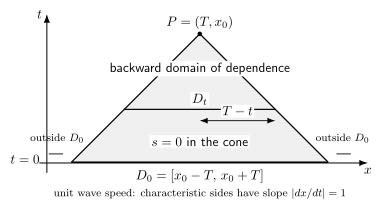
For unit wave speed, $P=(T,x_0)$ can depend only on initial data in $D_0=[x_0-T,x_0+T]$ and sources inside its backward characteristic cone. In the source-free case, the shrinking-domain flux identity prevents energy from entering through the null sides. Schematic 1+1-dimensional section.

Operationally, a localized source pulse and an array of detectors test this domain of influence by arrival times. The characteristic cone bounds the earliest possible influence; a particular source need not excite a nonzero signal at every allowed event. A smooth packet peak can also be delayed or reshaped. When a singular leading edge is present, it propagates along the characteristic geometry.

Checks and limitations

• Restoring a constant speed $v$ in $\partial_t^2-v^2\nabla^2$ changes the cone to $|\Delta\mathbf x|=v|\Delta t|$.
• Adding $m^2\psi$ changes neither the principal symbol nor the front speed.
• Energy conservation requires accounting for boundary flux. A reflecting wall and an open boundary are different problems.
• Characteristics determine possible propagation of singularities; they do not say that every solution has support on the cone. In three spatial dimensions the massless Green function has sharp cone support, while other dimensions or lower-order terms can produce interior tails.

Transfer task: a massive wave

For

$$(\partial_t^2-v^2\partial_x^2+m^2)\psi=0,$$

find the characteristics and explain what the mass changes.

Solution

The principal polynomial is $p=-\omega^2+v^2k^2$; $m^2$ is lower order. Thus the characteristic curves are

$$x\pm vt=\text{constant}.$$

A Fourier mode instead obeys $\omega^2=v^2k^2+m^2$, so

$$|v_{\rm g}|=\frac{v^2|k|}{\sqrt{v^2k^2+m^2}}\lt v$$

for finite $k$. The mass changes dispersion and the interior profile of the response, but it does not move the causal front outside $|x-x_0|=v|t-t_0|$. Interior support is not caused by mass alone: even the massless retarded fundamental solution in one spatial dimension has support inside the cone.

Boundary conditions and energy flux

Let $s=0$ on an interval $0\leq x\leq L$. Show that either fixed-end data $\psi=0$ or free-end data $\partial_x\psi=0$ conserve the interval energy. Then find the sign of the flux at $x=L$ for a purely right-moving wave $\psi=f(x-t)$.

Solution

Integrating the local balance law gives

$$\frac{dE_{[0,L]}}{dt}=S(0)-S(L), \qquad S=-\partial_t\psi\,\partial_x\psi.$$

For fixed ends, differentiating $\psi(t,0)=\psi(t,L)=0$ in time gives $\partial_t\psi=0$ at the boundaries, so $S=0$. For free ends, $\partial_x\psi=0$ there, again giving $S=0$. Both conditions conserve energy.

For $\psi=f(x-t)$, $\partial_t\psi=-f'$ and $\partial_x\psi=f'$, hence

$$S(L)=(f')^2\geq0.$$

Positive $S(L)$ is outward flux through the right endpoint, so the energy remaining in the interval decreases.

Continue to Fourier Modes, Dispersion, and Group Velocity to separate this front velocity from the motion of a narrowband envelope.

References

• Ethan Jaffe, “Lecture 21: Forward Fundamental Solution to the Wave Equation,” MIT 18.155 Differential Analysis, §§0 and 5–6, pp. 1 and 4–5, Massachusetts Institute of Technology, 2016. Official PDF.
• Sung-Jin Oh, Lectures on Wave Equation, §§1–4.2, pp. 1–10, University of California, Berkeley, 2014. Official PDF.