Sandwich Waves and Geodesic Response

A sandwich plane wave has curvature confined to a finite interval of null time. Before and after the wave, the Brinkmann metric can be flat, yet the map from incoming to outgoing geodesic separation data need not be the identity. The exact transfer matrix distinguishes displacement, velocity, and coordinate effects without importing a weak-field strain interpretation.

Required background. Frames, Coframes, and Anholonomy supplies parallel screen frames; Affine and Variational Geodesics supplies Jacobi fields and conjugate points.

Helpful background. Einstein’s Equation supplies the trace-free vacuum condition; The Riemann Curvature Tensor fixes the tidal matrix; Exact Solutions of Einstein’s Equations supplies the plane-wave family; The Wave Equation and Characteristics supplies finite wave packets.

Compact profile and Jacobi equation

Consider the four-dimensional Brinkmann metric

$$ds^2=-2\,du\,dv+\delta_{ij}dx^idx^j +A_{ij}(u)x^ix^j\,du^2,$$

where $x^i=(x,y)$, $A_{ij}=A_{ji}$, and $A(u)=0$ outside $u_-<u<u_+$. In vacuum, $\operatorname{tr}A=0$. Along any geodesic that crosses the wave, $du/d\lambda$ is a nonzero constant, so the affine parameter may be rescaled to $u$; a prime below means $d/du$. Geodesics tangent to the parallel null direction $\partial_v$ do not cross the profile and are not the probes considered here.

For neighboring crossing geodesics, their transverse separation $\xi$ in the parallel Brinkmann screen obeys

$$\xi''=A(u)\xi, \qquad R_{uiuj}=-A_{ij}(u).$$

This equation is exact: no small-amplitude or slowly varying assumption has been made. The curvature identity is also an independent check on the response sign. In a fixed screen direction with constant diagonal $A$, a positive entry produces hyperbolic separation while a negative entry produces oscillatory focusing; a rotating, time-dependent polarization requires the full matrix evolution.

Introduce fundamental matrices $P(u)$ and $Q(u)$ satisfying

$$P(u_-)=I,\qquad P'(u_-)=0, \qquad Q(u_-)=0,\qquad Q'(u_-)=I.$$

Then

$$\xi(u)=P(u)\xi_-+Q(u)\xi'_-.$$

The four blocks at any $u$ form the phase-space transfer matrix

$$\mathcal M(u)= \begin{pmatrix} P&Q\\ P'&Q' \end{pmatrix}, \qquad J= \begin{pmatrix} 0&I\\ -I&0 \end{pmatrix}.$$

Because $A$ is symmetric, $\mathcal M^T J\mathcal M=J$. In block form,

$$\begin{gathered} P^TP'=P'^TP,\qquad Q^TQ'=Q'^TQ,\\ P^TQ'-P'^TQ=I. \end{gathered}$$

Thus $\det\mathcal M=1$: phase-space information is preserved even when $\det P=0$ and a transverse congruence focuses. These identities are sensitive checks on analytic or numerical propagation.

What remains after the pulse

For probes initially comoving, $\xi'_-=0$, the outgoing data are

$$\xi_+=P_+\xi_- , \qquad \xi'_+=P'_+\xi_-.$$

If $P_+\neq I$, the pair has an exit displacement relative to its unperturbed continuation. That offset remains constant only when $P'_+=0$. If $P'_+\neq0$, the pair instead leaves with changed relative velocity, so its separation continues to evolve linearly in the flat after-zone. A special profile can make either effect vanish while leaving the other. Calling both simply “memory” hides this distinction.

At weak amplitude and with $\xi'_-=0$, holding $\xi\simeq\xi_-$ inside the integral gives the first-order estimate

$$\Delta\xi'\simeq \left(\int_{u_-}^{u_+}A(u)\,du\right)\xi_-.$$

If this integral vanishes, the exact response need not vanish: the matrices $A(u_1)$ and $A(u_2)$ act on an already evolved separation, and higher-order time-ordered contributions can remain. Exact propagation is therefore the appropriate discriminator.

Coordinate effects and focusing

In Rosen coordinates, initially fixed transverse labels can represent the reference congruence itself. Its metric $\gamma=E^TE$ may retain a changed scale or derivative after the profile, and the Rosen chart may fail when $\det E=0$ even though the Brinkmann curvature remains bounded. Neither a changing Rosen coordinate distance nor a Rosen-coordinate caustic alone is an invariant detector output.

The invariantly specified experiment is: choose the same incoming geodesics, parallel screen frame, affine normalization, and initial Jacobi data; propagate through the exact curvature; then compare the outgoing Jacobi vector and derivative in the continued parallel frame. A constant rotation of the screen conjugates the transfer blocks but does not change their eigenvalues or focusing condition.

Plane and sandwich waves in the exact-solution setting are reviewed in Bičák 2000, §8, printed pp. 66–76, Open PDF. The smooth-profile construction also supplies the controlled route to an impulsive limit described by Podolský 2002, §§3.3–3.3.1, arXiv manuscript pp. 10–12, Open PDF.

Worked square pulse

Translate $u$ so the pulse occupies $0<u<L$, and take $A=\operatorname{diag}(\kappa^2,-\kappa^2)$ there and zero elsewhere. Write

$$a=\kappa L,\qquad C=\cosh a,\quad S=\sinh a,\quad c=\cos a,\quad s=\sin a.$$

For the state $Z=(\xi_x,\xi_y,\xi'_x/\kappa,\xi'_y/\kappa)^T$, exact matching at the two edges gives

$$Z_+= \begin{pmatrix} C&0&S&0\\ 0&c&0&s\\ S&0&C&0\\ 0&-s&0&c \end{pmatrix}Z_-.$$

In particular, for initially comoving separation,

$$P_+=\operatorname{diag}(\cosh\kappa L,\cos\kappa L), \qquad P'_+=\operatorname{diag}(\kappa\sinh\kappa L,-\kappa\sin\kappa L).$$

One transverse direction defocuses while the other focuses. For an incoming circle

$$\xi_-=r_0(\cos\phi,\sin\phi),\qquad \xi'_-=0,$$

the exit data are

$$\xi_+=r_0(C\cos\phi,c\sin\phi), \qquad \xi'_+=\kappa r_0(S\cos\phi,-s\sin\phi).$$

At $a=\pi/2$, $P_+$ has rank one: the second Jacobi factor vanishes at the exit, but $\xi'_{+,y}=-\kappa r_0\sin\phi$ is generally nonzero, so the congruence immediately reopens.

The square profile is an idealization. Its $A$ and $R_{uiuj}=-A_{ij}$ have finite jumps at the edges, but no delta-function transverse tidal impulse: $\xi$ and $\xi'$ remain continuous while $\xi''$ jumps. Standard smooth approximants to the step converge to the same transfer matrix. An exact square-pulse construction, including transverse matching, ring deformation, and line caustics, is developed in Chakraborty and Kar 2022, §§II.B–II.C and III.A, printed pp. 6–14, Open PDF.

The figure instead chooses $a=\kappa L=\pi/4$, so the exit map is nonsingular and the later flat-zone caustic can be followed explicitly.

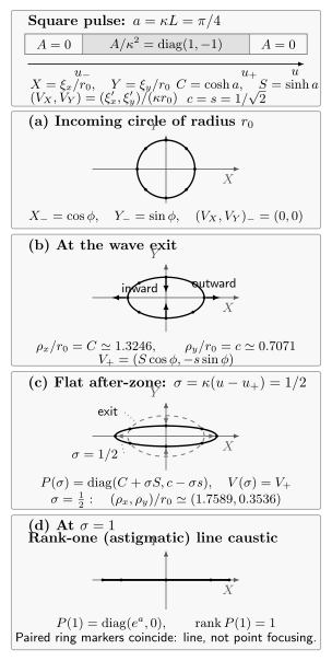
Exact Jacobi response for $A=\kappa^2\operatorname{diag}(1,-1)$, $\kappa L=\pi/4$, and an initially comoving circular family of radius $r_0$. At exit the semiaxes are $r_0\cosh(\pi/4)=1.3246r_0$ and $r_0/\sqrt2=0.7071r_0$, with $\xi'_+/(\kappa r_0)=(\sinh(\pi/4)\cos\phi,-\sin\phi/\sqrt2)$. In the flat after-zone, $\sigma=1/2$ gives $1.7589r_0$ and $0.3536r_0$; at $\sigma=1$ only the focusing Jacobi factor vanishes, so $\det P=0$ and the section forms a rank-one line caustic, not a point. The step profile has finite curvature jumps and no delta-function transverse tidal impulse. Ellipses are quantitative in the continued parallel screen; arrows show direction only.

For $\sigma=\kappa(u-u_+)\ge0$, propagation in the flat after-zone gives the complete initially comoving map

$$P(\sigma)= \operatorname{diag}(C+\sigma S,c-\sigma s).$$

At $a=\pi/4$ and $\sigma=1/2$, its semiaxes are $r_0(C+S/2)=1.7589r_0$ and $r_0(c-s/2)=0.3536r_0$. At $\sigma=1$,

$$P(1)=\operatorname{diag}\left(e^{\pi/4},0\right).$$

The image of the initial disk has therefore collapsed in one direction but not the other: this is an astigmatic, rank-one line caustic, not point focusing. The full phase-space map remains symplectic and invertible, so the caustic is not a curvature singularity.

Exercises

Show that $W=P^TQ'-P'^TQ$ remains equal to the identity, and derive the other two independent block identities in $\mathcal M^TJ\mathcal M=J$.

Solution

Differentiate and use $P''=AP$, $Q''=AQ$:

$$W'=P^TAQ-(AP)^TQ=0$$

because $A^T=A$. At $u_-$, the initial data give $W=I$. Applying the same calculation to $P^TP'-P'^TP$ and $Q^TQ'-Q'^TQ$ shows that both are constant; their initial values vanish. These are exactly the three independent block conditions in $\mathcal M^TJ\mathcal M=J$.

For the $a=\pi/4$ pulse, derive the first after-zone caustic time and determine whether the incoming circular section becomes a point or a line.

Solution

The two Jacobi factors are

$$p_x(\sigma)=C+\sigma S, \qquad p_y(\sigma)=c-\sigma s.$$

For $\sigma\ge0$, $p_x>0$. Since $c=s=1/\sqrt2$ at $a=\pi/4$, $p_y=0$ first at $\sigma=c/s=1$. Thus $P(1)=\operatorname{diag}(e^{\pi/4},0)$ has rank one. A point $r_0(\cos\phi,\sin\phi)$ on the incoming circle maps to $(r_0e^{\pi/4}\cos\phi,0)$, a line segment. It does not map to a point because the defocusing Jacobi factor never vanishes.

References

• Bičák, Jiří. “Selected Solutions of Einstein’s Field Equations: Their Role in General Relativity and Astrophysics.” In Einstein’s Field Equations and Their Physical Implications, edited by Bernd G. Schmidt, 1–126. Lecture Notes in Physics 540. Berlin: Springer, 2000. DOI; Open PDF.
• Chakraborty, Indranil, and Sayan Kar. “A Simple Analytic Example of the Gravitational Wave Memory Effect.” The European Physical Journal Plus 137 (2022): 418. DOI: 10.1140/epjp/s13360-022-02593-y; Open PDF.
• Podolský, Jiří. “Exact Impulsive Gravitational Waves in Spacetimes of Constant Curvature.” In Gravitation: Following the Prague Inspiration, edited by Oldřich Semerák, Jiří Podolský, and Martin Žofka, 205–246. Singapore: World Scientific, 2002. DOI; Open PDF (arXiv manuscript).